Elemental mapping (EDS)
Elemental mapping (EDS)
One of elemental analysis methods using characteristic X-rays generated by an electron-beam. The method visualizes the distribution of the constituent elements in the specimen by two-dimensionally displaying the characteristic X-ray intensities or the concentrations of the elements.
In elemental mapping using energy-dispersive X-ray spectroscopy (EDS), an electron beam is two-dimensionally scanned over a specimen area, and the characteristic X-ray spectra generated by the electron beam are acquired pixel by pixel. From those spectra, the X-ray intensities or the calculated concentrations of the target elements are displayed pixel by pixel, to acquire an elemental map (Fig. 1).
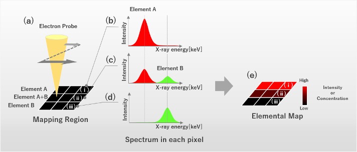
Fig. 1 Procedure of elemental mapping.
- (a) By two-dimensionally scanning an electron beam over an area where element A and element B exist, the X-ray spectra generated from each pixel are acquired.
- (b) Spectrum acquired from pixel (i) in Fig.(a). A strong characteristic X-ray peak of element A is depicted.
- (c) Spectrum acquired from pixel (ii) in Fig.(a). Characteristic X-ray peaks of element A and element B are depicted.
- (d) Spectrum acquired from pixel (iii) in Fig.(a). A characteristic X-ray peak of element B is depicted.
- (e) The integrated intensities of the characteristic X-rays of element A or the element concentrations of element A are plotted pixel by pixel to provide the elemental map of element A.
There are three types of elemental maps using EDS: Two are intensity maps of characteristic X-rays and the third is a concentration map of elements. The features of each map are presented in Table 1.
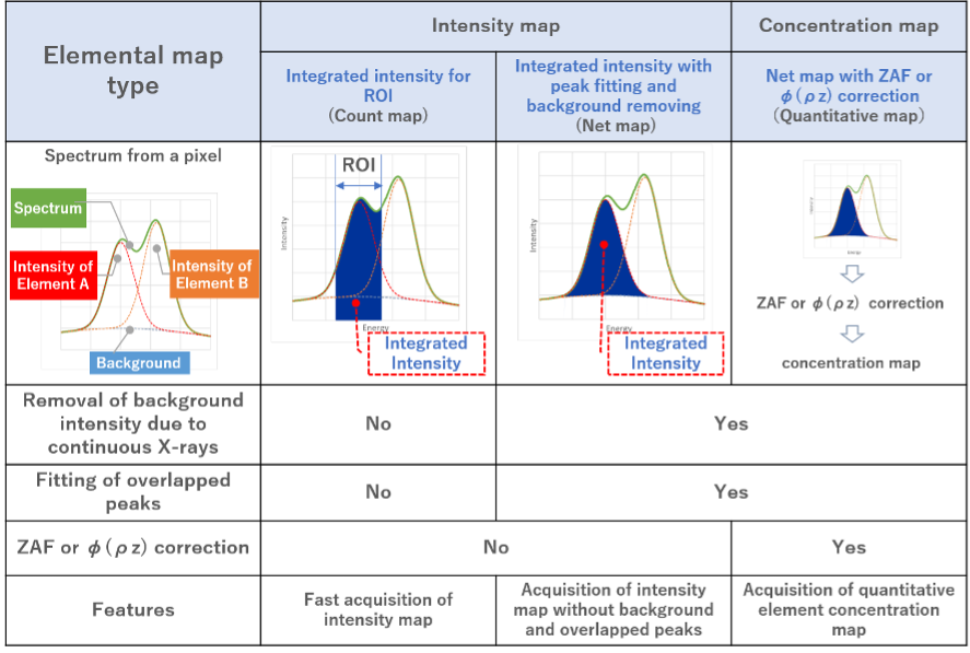
Table 1 Comparison of the three elemental maps using EDS.
1. Characteristic X-ray intensity map
The map displays the characteristic X-ray intensities of the target elements pixel by pixel. The intensity map qualitatively shows where the elements are more abundant. This is because the intensity of the characteristic X-rays detected under the same condition of electron-beam illumination is roughly proportional to the abundance of the elements.
There are two types of the intensity maps.
1) The first is to display the integrated intensity distribution for ROI (count map).
An energy region for integration (ROI: Region of Interest) is set for each element, and the value of the integrated intensity for ROI is displayed pixel by pixel. At JEOL, the map is called "count map". The advantage of the method is easy and quick to display the map.
However, since the energy resolution of EDS is approximately 130 eV (defined at Mn-Kα 5.9 keV), the ROI of the target element may overlap that of the other element, giving an incorrect elemental distribution. When the background intensities generated by continuous X-rays are largely different from pixel to pixel, the map may not correctly provide the differences of the characteristic X-ray intensities of neighboring pixels due to the large differences in the background.
2) The second is to display the integrated intensity distribution subjected to background removal and peak separation (net map).
This method improves the above method (1) to obtain a better accuracy of the element distribution. At JEOL, the map is called "net map".
The spectrum of a standard specimen with known mass concentrations of constituent elements is measured, and the background due to continuous X-rays is removed. Then, the standard spectrum is prepared. Next, the spectrum of an unknown specimen is measured, and the background due to continuous X-rays is also removed. Then, as shown in Fig. 2, the standard spectra of the two elements are each multiplied by a factor and the two spectra are combined. The values of the two factors are determined so as to best reproduce the spectrum of the unknown specimen. As a result, the overlapping spectra of the unknown specimen are separated into the spectra of the two elements.
By multiplying the factor calculated for each element (i.e. the ratio of the intensity of the spectrum of the unknown specimen to that of the standard spectrum) by the integrated intensity of the element of the standard specimen, the integrated intensity of the element of the unknown specimen is obtained. By performing the procedure for every pixel, the intensity distribution of the characteristic X-rays of the target element is obtained.
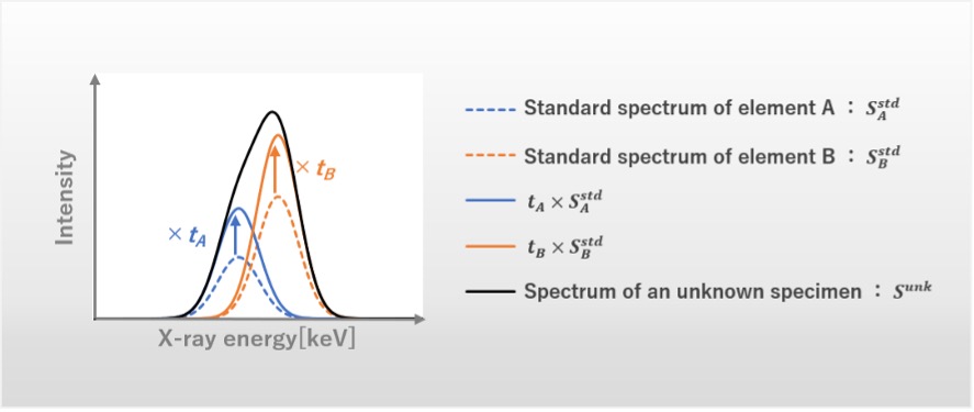
Fig. 2 Schematic diagram of peak separation.
1) Factors tA and tB, which reproduce the spectrum of the unknown specimen Sunk, is obtained from the equation
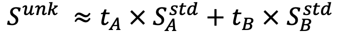 .
.2) The integrated intensities  from element A and element B of the unknown specimen are obtained from the equations
 ,
,where,  and
and  are the integrated intensities from element A and element B of the standard specimen, respectively.
2. Element concentration map (quantitative map)
This map displays the element concentrations of the target elements, called "quantitative map".
The element concentration map is obtained by the following procedures. First, the X-ray intensity of the spectrum for each pixel (p) is normalized so that it is the intensity obtained under the same measurement condition as the standard spectrum.
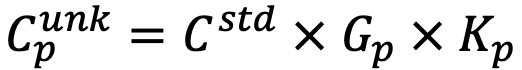
Next, the factor (tp) is obtained in the same way as for the net map. This factor obtained after normalization is the correct ratio of intensity from the standard specimen to that from the unknown specimen, called K ratio (Kp). Furthermore, the correction factor (Gp), which originates from the difference in X-ray intensities due to the different coexisting elements between the standard specimen and the unknown specimen, is calculated using the ZAF correction or the Phi-Rho-Z (φ(ρz)) method.
If the concentration of the standard specimen is Cstd, the element concentration of the unknown specimen  for each pixel (p) is obtained by the following equation.
(For details of Gp, refer to the related terms "quantitative correction", "ZAF correction" and "Phi-Rho-Z (φ(ρz)) method".)
Real analysis example: Intensity maps and concentration map of a SnPbBi alloy
The following analysis example demonstrates how the net map improves the count map.
Fig. 3(a) shows a compositional image of a SnPbBi alloy taken with backscattered electrons. X-ray spectra were measured from rectangular regions indicated by green, red and blue. A Sn spectrum was observed in the green region, a Pb spectrum in the red region, and a Bi spectrum in the blue region. The spectrum of Sn does not overlap with those of Pb and Bi, but spectra of Pb and Bi overlap to each other. Thus, in the count map, which integrates the ROI intensities, the regions containing Pb and Bi are mixed up and not separated.
On the other hand, in the net map where peak separation is applied, the regions of Pb and Bi are clearly separated as shown in the center column of Fig. 4. The concentration map is shown in the right column of Fig. 4 for comparison. In the present case, the concentration map is almost the same as the net map, but the concentration map can show quantitative or gradual change of the element concentrations using a color scale.
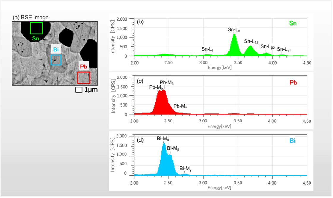
Fig. 3 Backscattered electron image of a SnPbBi alloy and its X-ray spectra.
- (a) Backscattered electron compositional image of a SnPbBi alloy.
- (b), (c), (d) X-ray spectra respectively measured from areas of green, red and blue in Fig.(a).
Labels such as "Sn-Lα" are the characteristic X-rays designated by Siegbahn and represent the transitions of electrons. For example, "Sn-Lα" indicates the characteristic X-ray generated by the transition of an electron in the d-orbital of the M shell into a vacancy in the p-orbital of the L shell.
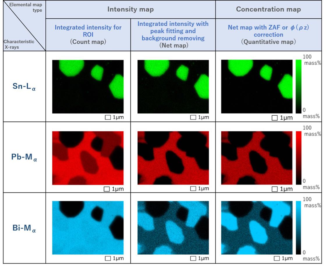
Fig. 4 Count maps (left column), Net maps (center column) and Quantitative maps (right column) of
Sn-Lα, Pb-Mα and Bi-Mα created by three methods.
Three type maps show no difference for the distribution of Sn.
The net map and quantitative map of Pb provide correctly the regions of Pb (red) and Pb-free regions (black). However, the count maps of Pb show some of the Pb-free regions as if they contain some Pb (dark red) because the characteristic X-rays from Bi are also captured.
The net map and quantitative map of Bi distinguish correctly the regions of large Bi concentrations (blue), the regions of small Bi concentrations (dark blue) and the Bi-free regions (black). However, the count map of Bi scarcely distinguish blue and dark blue regions because the map also takes in characteristic X-rays from coexisting Pb.
However, it is noted that the present example unfortunately does not show the continuous change as represented by the color scale in the quantitative map.
Appendix
Example of intensity maps and concentration map of a mineral specimen containing Fe.
The net map and the quantitative map often exhibit similar elemental distributions because the characteristic X-ray intensity generated is roughly proportional to the concentration of an element. However, in some specimens, the net map and the quantitative map may be different due to the absorption effect of X-rays by the coexisting elements.
The following is an example of the study of a specimen consisting of two minerals with different contents of Fe.
Fig. 5 shows a backscattered electron compositional image of the specimen. The X-ray spectra were acquired from the dark region on the left side (region A) and from the light region on the right side (region B). It was found that region A is composed of Fe, Mn and O, while region B is composed of Fe and S. The result of quantitative analysis with ZAF correction shows that the concentration of Fe in region A is higher than that in region B.
Fig. 6 shows two types of intensity maps and a concentration map acquired from the regions A and B. The two intensity maps (left and center) show that the characteristic X-ray intensity of Fe in region B is higher than in region A. On the other hand in the concentration map (right), the concentration of Fe in region A is higher than region B. The result indicates the importance of ZAF correction in this case.
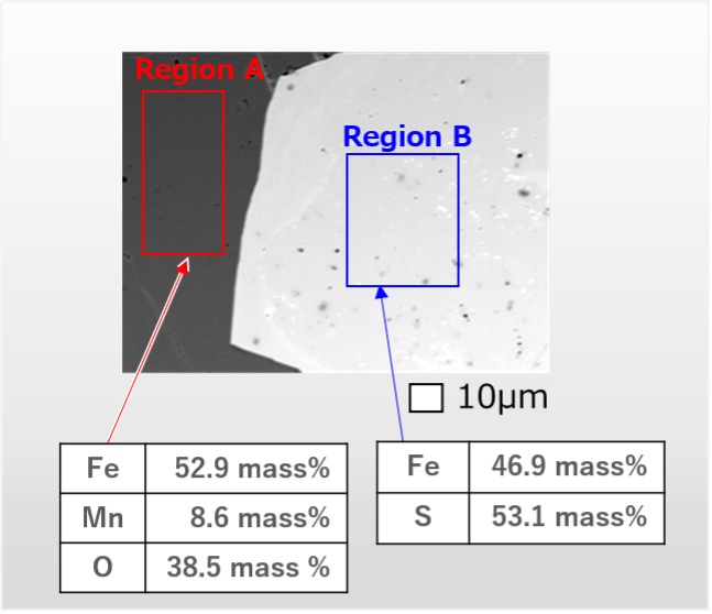
Fig. 5 Backscattered electron compositional image of a mineral specimen.
Two tables show the result of quantitative analysis with ZAF correction. The concentration of Fe in region A is higher than in region B.
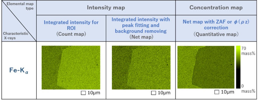
Fig. 6 Elemental maps of Fe obtained by the three methods.
The regions where the X-ray intensities or element concentrations of Fe-Kα are high and low are shown respectively by light green and dark green.
The count map and net map (left and center) show higher intensities in the right region, but the quantitative map (right) exhibits a lower concentration in the right region.
Related Term(s)
Term(s) with "Elemental mapping (EDS)" in the description
Are you a medical professional or personnel engaged in medical care?
No
Please be reminded that these pages are not intended to provide the general public with information about the products.