Structural Analysis of Organic Compound Using 2D - NMR Spectrum
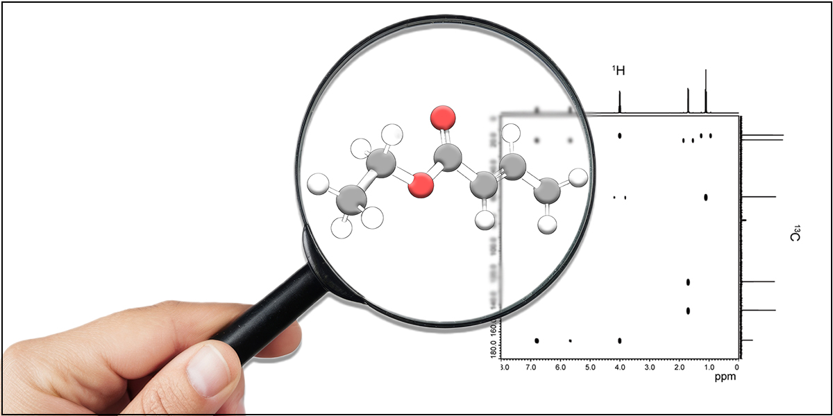
In this column, we will explain the structural analysis of organic compound by using 2D-NMR spectrum.
Structural Analysis of one-dimensional NMR (1D-NMR)
One-dimensional NMR (1D-NMR) is the most basic measurement of NMR spectroscopy, in which the spectrum is displayed along a horizontal axis (chemical shift). As introduced in the previous column, information on chemical shift, integration ratio, and splitting pattern (coupling) is used to analyze the structure of an object. However, it can be difficult to perform structural analysis using only 1D-NMR data when the number of detected signals is large, when signals appear in overlapping positions, or when couplings are complex.
The two-dimensional (2D-NMR) spectral analysis method introduced in this column can be used extensively regardless of the object to be analyzed, since the basic sequence of steps is followed. In addition, by following the basic procedures, even beginners can mechanically perform structural analysis.
Related article
How to read NMR spectra from the basics (chemical shift, integration ratio, coupling)
What is 2D-NMR?
2D-NMR is a method used to check a more detailed molecular structure than 1D-NMR.
Since there are many 2D-NMR measurement methods, here, we introduce representative measurement methods.
| Measurement Name | What you can find out |
|---|---|
| COSY | A method to observe coupling between neighboring same nuclides (frequent:1H/1H) |
| INADEQUATE | A method to observe coupling between neighboring 13Cs |
| HMQC/HSQC | A method to observe coupling of a directly coupled heterogeneous nuclei (frequent: 1H/13C) |
| HMBC/H2BC | A method to observe the correlation signals of heterogeneous nuclei(frequent: 1H/13C) via 2-3 bonds |
| ADEQUATE | A method to detect 13C-13C coupling by 1H observation |
| NOESY/ROESY | A method to observe the correlation signals between 1Hs that are closely located(with NOE interaction) |
Structural Analysis Using J Coupling Correlation
This time we introduce an example of structural analysis using "J Coupling Correlation" which is an interaction via chemical bonding. Structural analysis of an object is conducted by following the 4 steps below.
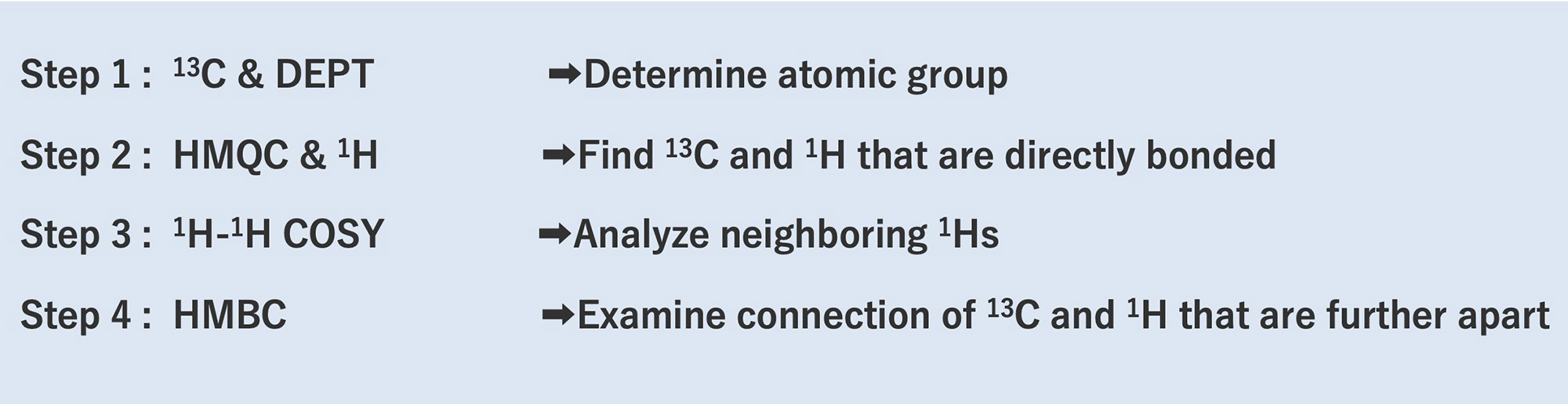
In Step 1, we use a 1D-NMR spectrum of 13C and DEPT to determine and estimate the atomic group and functional group.
In Step 2, we use HMQC and 1D spectrum of 1H to find 13C and 1H that are directly bonded.
In Step 3, we use COSY to examine and locate which is the neighboring 1Hs.
By using information obtained in Step 2 and 3, substructures can be determined to some extent.
In Step 4, we use HMBC to determine the structure of the remaining parts, by considering the connection of 13C and 1H which are further apart.
Structural analysis example of C 6H10O2
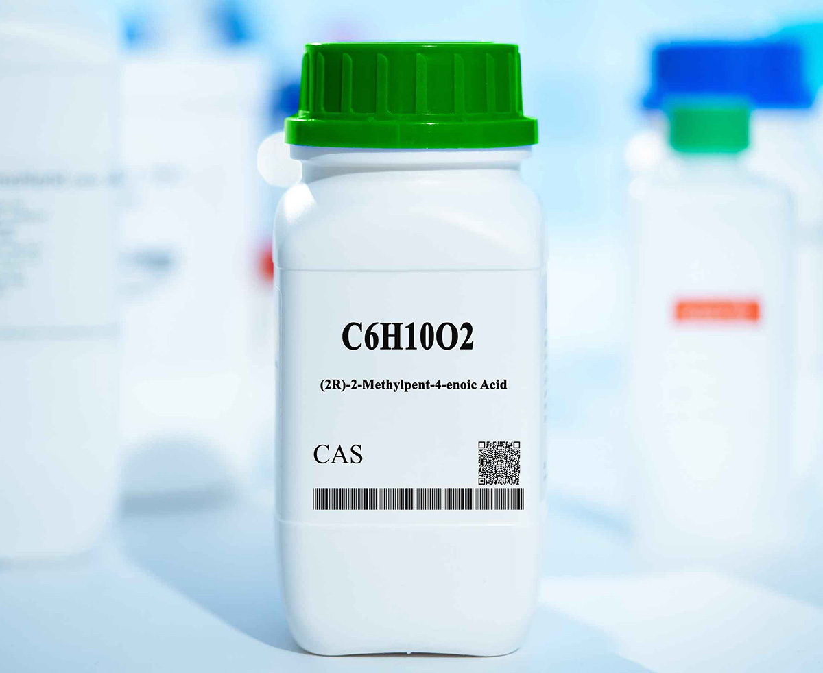
Now we will explain the structural analysis of a specific sample.
This time, we use a substance whose molecular formula C6H10O2 is only known and dissolve in heavy chloroform.
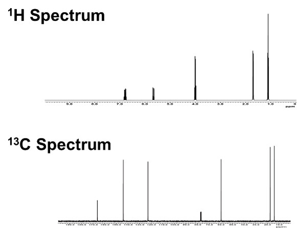
Step 1 13C (1D-NMR) & DEPT
In Step 1, we use a 1D-NMR spectrum of 13C and DEPT to determine and estimate atomic group and functional group. First, as shown in Fig. 1, we put a symbol on each signal in 1D-NMR spectrum of 13C. Starting with the signal on the right side of the spectrum, from the high-field side, add symbols A, B, C... and so on. The chemical shift of each signal is read to one decimal place. The read information is summarized in Table 1.
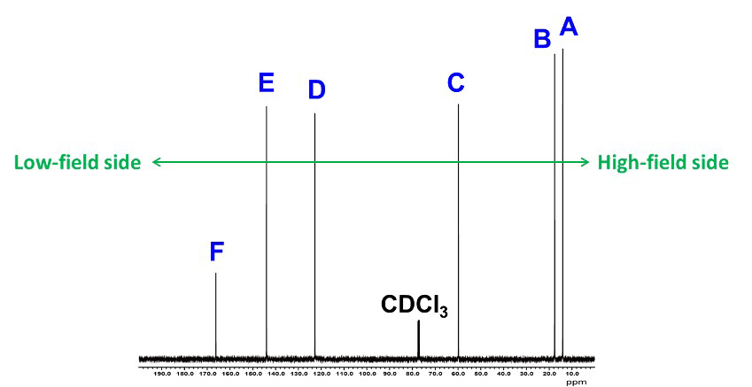
Fig. 1 13C Spectra of C6H10O2
Table 1 13C Spectra Information
| Signal | Chemical Shift |
|---|---|
| A | 14.1 ppm |
| B | 17.6 ppm |
| C | 59.8 ppm |
| D | 122.8 ppm |
| E | 144.0 ppm |
| F | 166.2 ppm |
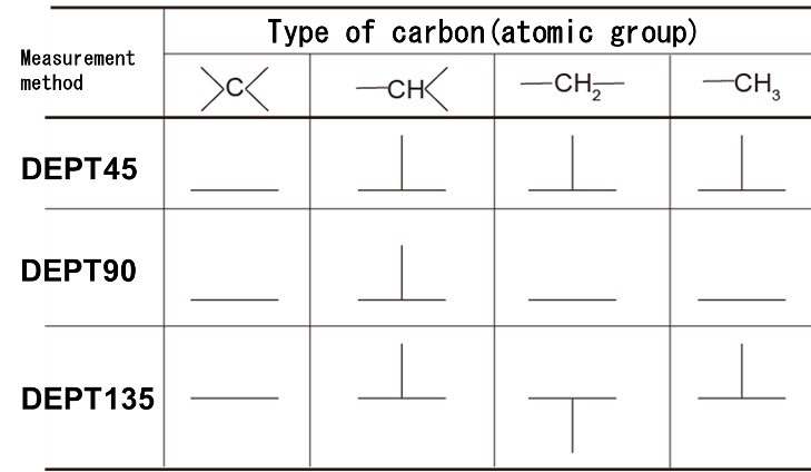
Next, we will confirm the results of the DEPT spectra. Since DEPT observes the carbon to which hydrogen is directly bonded, the series of the carbon atom of interest (the number of hydrogen directly bonded to the carbon of interest) is known. In other words, it is possible to identify atomic groups such as CH3, CH2, and CH. (DEPT cannot detect spectra of quaternary carbons.) DEPT provides three types of spectra, depending on the measurement parameters (DEPT135, DEPT90, and DEPT45).
Table 2 lists the signal appearance patterns in the three types of DEPT spectra. In DEPT135, the signals of CH3 and CH are detected upward, while the signal of CH2 appears downward (opposite phase). It is often possible to discriminate CH3 or CH from the chemical shift. In many cases, the DEPT135 measurement alone is sufficient. If discrimination by DEPT135 alone is difficult, measure DEPT90, in which only the signal of CH is detected.
Table 2 DEPT Signal Appearance Patterns
We will use the DEPT spectra to determine the atomic groups of the sample. As shown in Figure 2, we will discriminate the atomic groups of each signal by comparing the signal appearance patterns of the 1D-NMR spectrum of 13C and the DEPT spectrum.
-----
DEPT135・・・Upward signal: CH3 or CH, Downward signal: CH2
DEPT90・・・ Detectable signal : CH
Signal detected only in the 1D-NMR spectrum of 13C and not detected in the DEPT spectrum: quaternary carbon
-----
Using the information so far, we were able to determine that the atomic groups of each signal are, from right to left, A (CH3), B (CH3), C (CH2), D (CH), E (CH), and F (quaternary carbon).
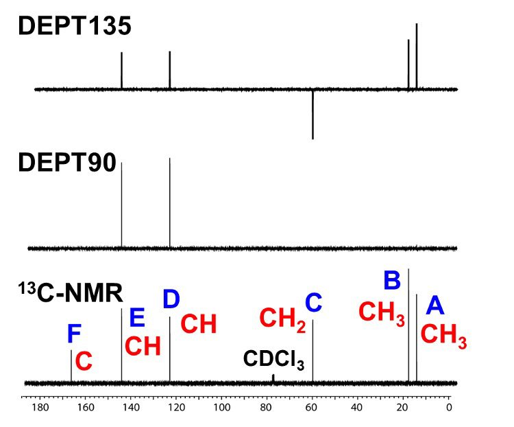
Fig. 2 13C Spectra and DEPT Spectra of C6H10O2
The information so far is summarized in Table 3. This information is used to estimate the atomic groups and functional groups.
Table 3 13C Spectra Information (2)
| Signal | Chemical Shift | Atomic Group |
|---|---|---|
| A | 14.1 ppm | CH3 |
| B | 17.6 ppm | CH3 |
| C | 59.8 ppm | CH2 |
| D | 122.8 ppm | CH |
| E | 144.0 ppm | CH |
| F | 166.2 ppm | C |
Figure 3 shows the chemical shift table for 13C. At an approximate border of 100 ppm, the saturated carbon signals are appeared on the right and the unsaturated carbon signals on the left. We will compare the information summarized in Table 3 with the chemical shift table. First, if we look at D (122.8 ppm) and E (144.0 ppm), we see that they are in the region of unsaturated carbon, indicating that this CH is derived from unsaturated carbon. Next, if we look at F, the chemical shift value is 166.2 ppm, which is in the ester region. The molecular formula of this substance is C6H10O2, and since there are two Os, the quaternary carbon of F is presumed to be derived from the COO group.
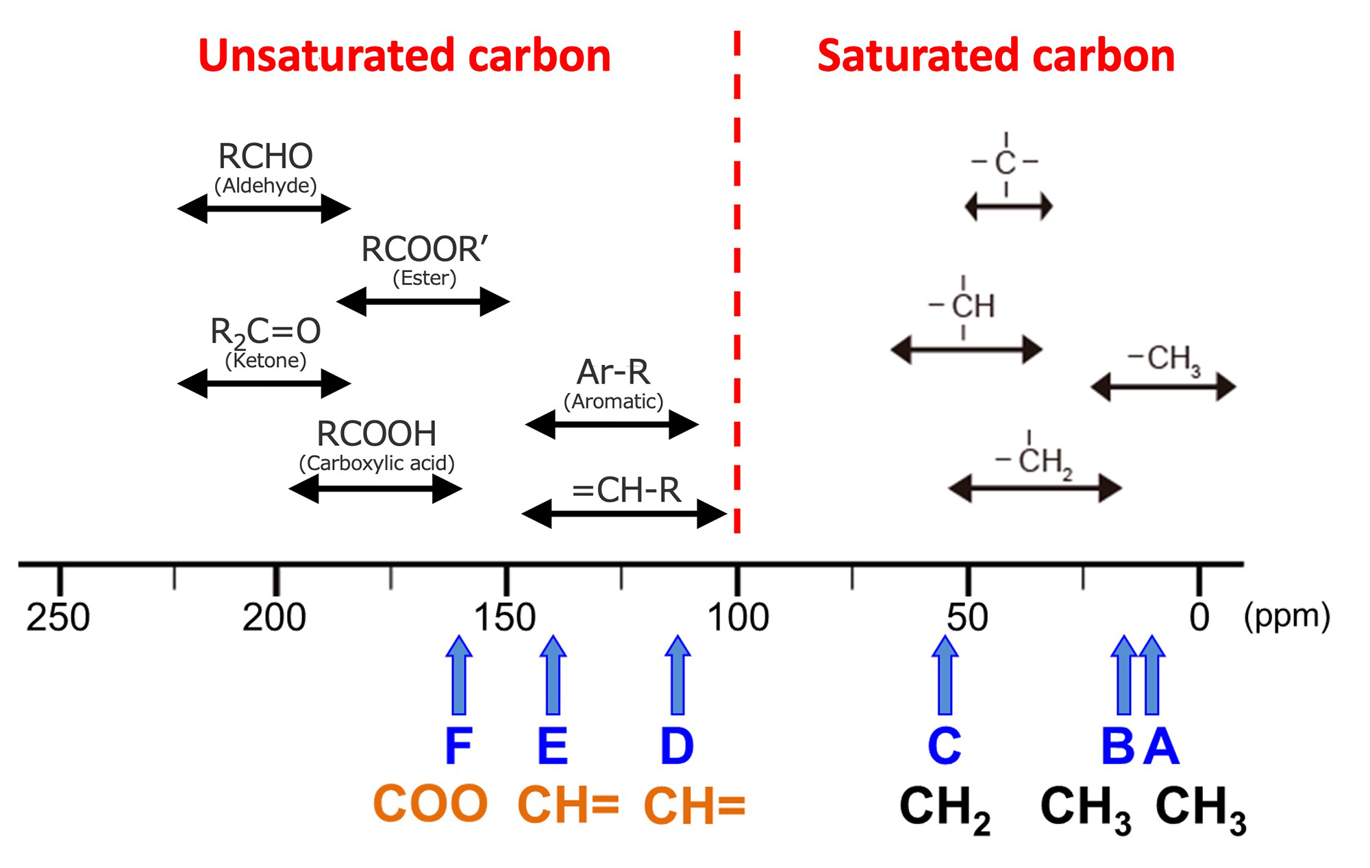
Figure 3 13C Chemical Shift Table
The information so far is summarized in Table 4.
Table 4 13C Spectra Information (3)
| Signal | Chemical Shift | Atomic Group |
|---|---|---|
| A | 14.1 ppm | CH3 |
| B | 17.6 ppm | CH3 |
| C | 59.8 ppm | CH2 |
| D | 122.8 ppm | CH= |
| E | 144.0 ppm | CH= |
| F | 166.2 ppm | COO |
Step 2 HMQC & 1H
In Step 2, we will use HMQC and 1D-NMR spectra of 1H to find directly bonded 13C and 1H combinations. HMQC will tell you the combination of 1H and 13C that are directly bonded. Spin couplings are written with a symbol, such as 1JCH. The number of bonds is written in the upper left corner of the J representing the spin coupling, and the nucleus to which it is bound is written in the lower right corner of the J.
Figure 4 shows an HMQC spectrum. In a 2D-NMR spectra, a high-resolution 1D-NMR spectrum is displayed at each axis; for HMQC, the 1H spectrum is displayed on the X-axis and the 13C spectrum on the Y-axis. In Step 2, the same symbols that were attached to each signal in the 13C spectrum in Step 1 are attached to the signals in the 13C spectrum on the Y-axis, with the upper side of the Y-axis representing the high-field side (small chemical shift) and the lower side representing the low-field side (large chemical shift).
Next, draw a line from the 13C signal on the Y-axis to the HMQC correlation signal and confirm which 1H is directly bonded to 13C. For example, if we focus on the 13C signal of C, we draw a line toward the side, and when the line hits the correlation signal, we draw a line up from there. The 1H signal that we have reached here is the counterpart directly bonded to signal C of 13C. When the corresponding 1H is found in this way, the 1H is marked with the same symbol as the counterpart 13C. Since it is the counterpart of the signal C of 13C, we will also put the symbol C on this 1H. All correlated combinations will be given a similar symbolization.
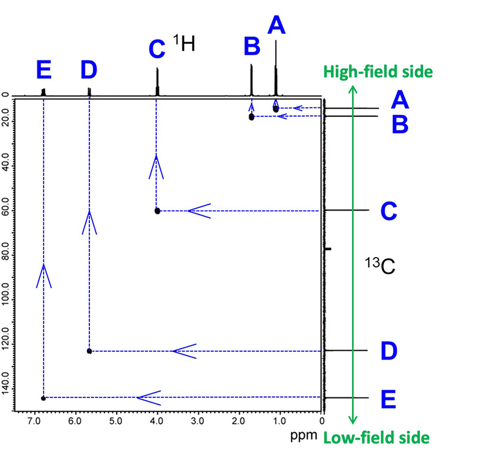
Fig.4 HMQC Spectra
Step 3 1H-1H COSY
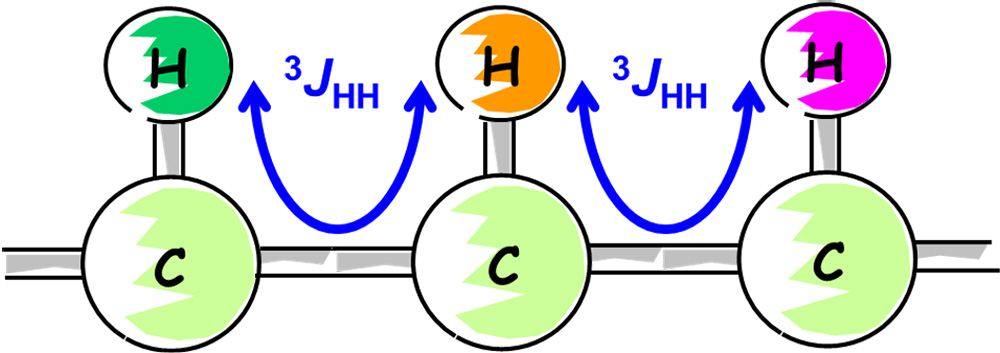
Fig. 5 Correlation of 1Hs via Three Bonds
In Step 3, we will use 1H-1H COSY to see which are the neighboring 1Hs. COSY shows the spin-coupled 1H connections. What can be observed mainly is the correlation between 1Hs via three couplings, as shown in Figure 5. In symbols, we denote this as 3JHH.
As shown in Fig. 5, if 1Hs in a 3JHH relationship are lined up, we can follow the 1H connections one after another.
In COSY, in addition to the 3JHH, a 2JHH through two couplings and a remote 4JHH can also be observed.
However, the most important and necessary information is the correlation between 1Hs at the neighboring 13C, 3JHH.
Fig. 6 shows the actual COSY spectra. COSY shows 1H spectra both on the X-axis and Y-axis.
In Step 1, we assigned a symbol to each 13C signal. In Step 2, we assigned a symbol to each 1H signal that is directly coupled to 13C using HMQC. In Step 3, we first assigned the same symbols to the signals in the 1H spectrum on the X and Y axes as we did in Step 2. We looked at the HMQC spectra we used earlier (Figure 4) and copied the symbols attached to the signals in the 1H spectra on the X-axis as they were.
Note that in Figure 6, the symbols are alphabetically ordered from the high-field side, but this just happened to be the case for this sample. The symbols on the 1H signal are not always in alphabetical order.
Also, in the COSY spectra, signals line up on the diagonal line (called diagonal signals) when the diagonal line is drawn. But these are not used as information for structural analysis. The off-diagonal signals are the COSY correlation signals.
We draw a line from the correlated signal toward the X- and Y-axes spectra and find the 1Hs that are spin-coupled to each other. For example, if we focus on the correlation signal circled in green, we find the 1H signal C on the X-axis and the 1H signal A on the Y-axis. Therefore, we can see that signals C and A are spin-coupled (neighboring) to each other. Once the counterpart is found, we add a symbol to the correlated signal. For example, C/A, to specify that they are 1H signals in a 3JHH relationship. Since the correlated signals of COSY appear in a line symmetric position with respect to the diagonal, we find the 3JHH counterpart in the same way for all correlated signals.
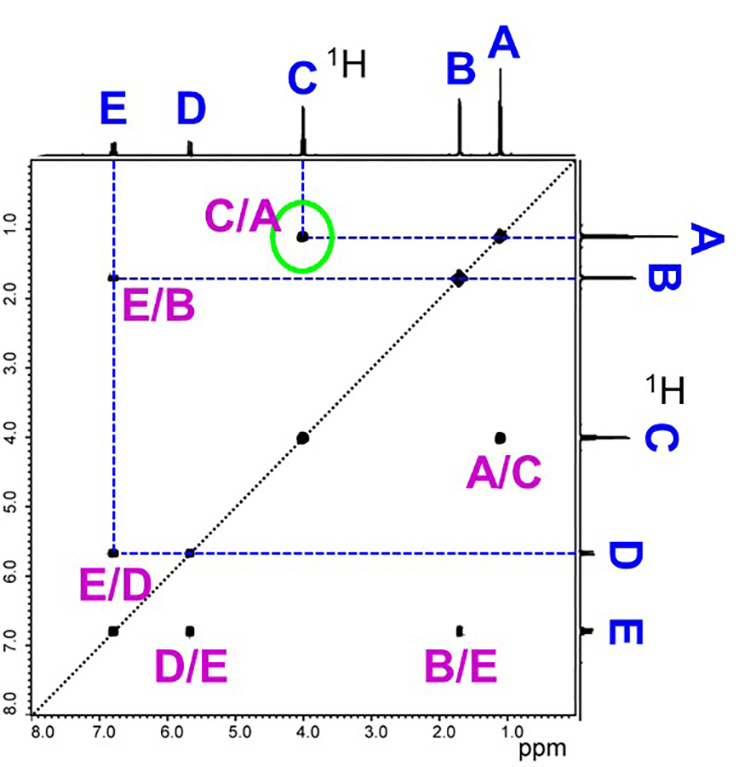
Fig. 6 COSY Spectra
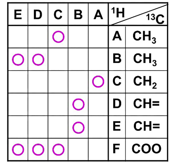
Once the information on the correlated signals of COSY is available, a correlation table for each signal is created.
Table 5 is the correlation table for COSY. Write the symbols for the 1H signals in vertical and horizontal order, as per the spectrum of the data on the 1H-1HCOSY axis. (In the case of this sample, they happen to be arranged alphabetically, but you should look at the COSY spectra and list them in chemical shift order.) For example, if the correlated signals are C and A, mark the intersection of C and A. In this way, all correlated signals are entered in the COSY correlation table.
Table 5 COSY Correlation Table
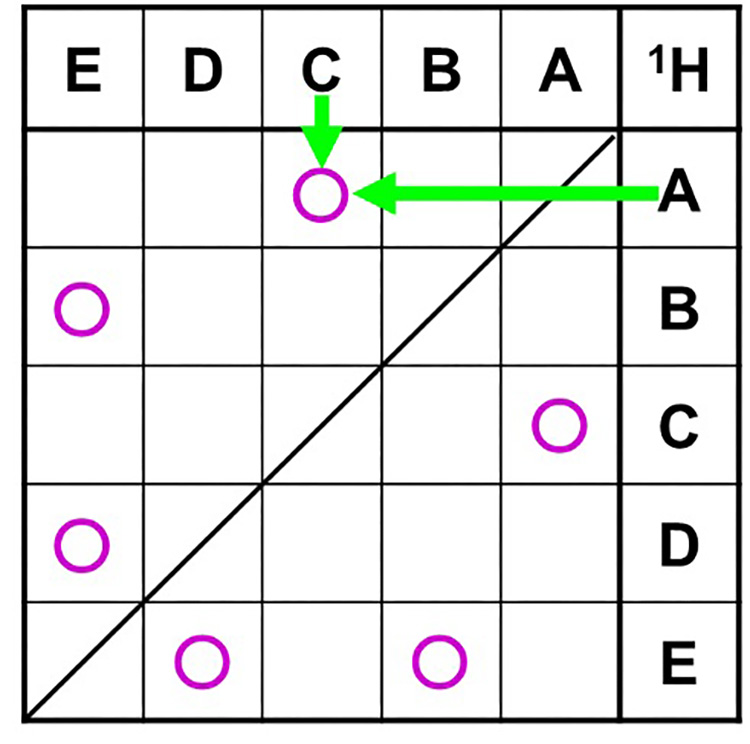
Fig.7 shows the diagram of correlation signal of COSY.
In this sample, COSY correlation signal was observed between 1H of C and 1H of A.
The HMQC spectra also indicated that 1H of C and 13C of C are directly coupled. In the same way, 1H of A and 13C of A are directly coupled.
Therefore, COSY correlation signals between C and A can induce that 13C of C and 13C of A are neighboring. In other words, using the COSY information, we can indirectly find the neighboring 13C connections from the neighboring 1H connections.
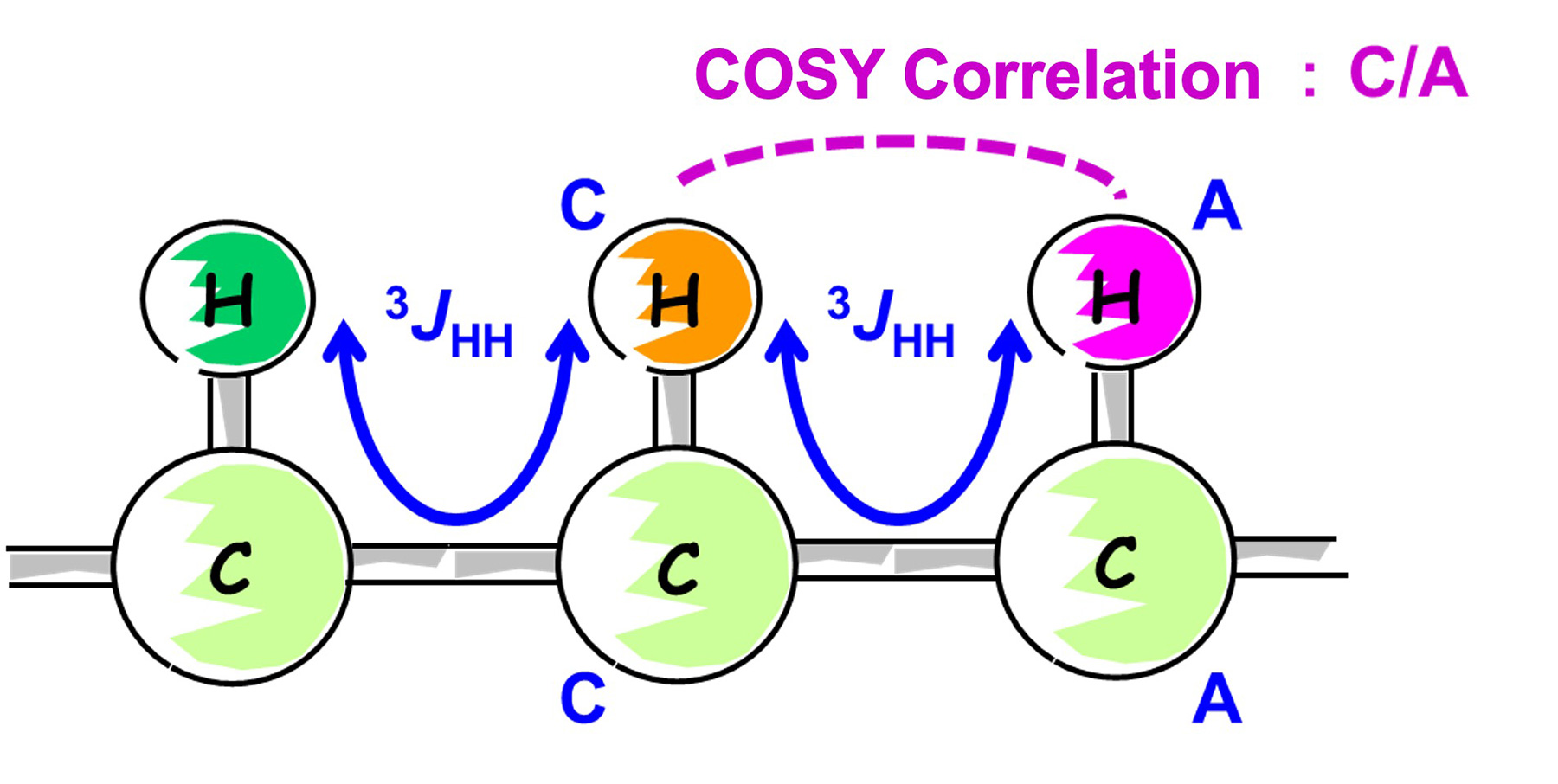
Fig. 7 COSY Correlation Signals
The information that we have so far is the 13C spectrum information (Table 4) and the COSY correlation table (Table 5). From the COSY correlation table, we can see that the carbon atoms derived from the 13C signals A-C, B-E, and D-E are neighboring to each other. Combined with the information from the 13C spectrum, when we rewrite the symbols as atomic groups, we have A-C : "CH3-CH2-", B-E-D : "CH3-CH=CH-", and F : "COO" in Step 1. Therefore, we know that this compound is composed of the following three substructures.
----
Substructure 1:CH3-CH2- ・・・ A-C
Substructure 2: CH3-CH=CH- ・・・ B-E-D
Substructure 3: COO ・・・ F
----
Next, we will consider what kind of molecule these will make by connecting each substructure (Figure 8). We will list all possible molecular structures from the combination of the three substructures. When considering molecular structures, it is easier to focus on the substructure containing CH3 because CH3 is located at the end of the structure. In this case, there are two possible structures. Firstly, Substructures 1 and 2 are found to be the ends of the molecular structure because they contain CH3.And since 1 and 2 are located at the ends, we can predict that substructure 3 is sandwiched between 1 and 2. The different orientations of substructure 3 allowed us to create two different inferred structures (I, II). The orientation of the COO can be used to determine which inferred structure is more reasonable. Therefore, HMBC measurements are performed to confirm the long-range spin coupling with respect to the COO.

Fig. 8 Combination of Three Substructures
Step 4 HMBC
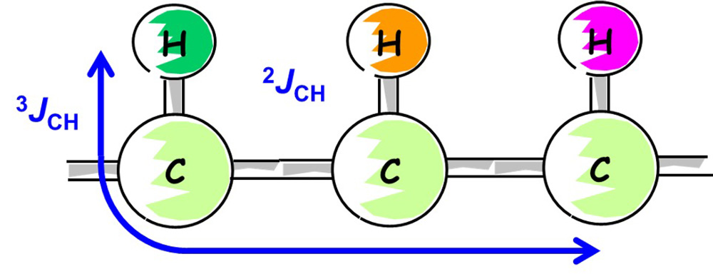
Fig. 9 CH Correlation through 2 or 3 Bonds
In Step 4, we will consider long-range spin coupling between 13C and 1H by using HMBC.
In HMBC, we can observe the correlations of 2JCH through two bonds or 3JCH through three bonds, as shown in Figure 9.
Fig. 10 is the actual spectra of HMBC. The HMBC axes are the same as HMQC's case, 1H spectra on X-axis and 13C spectra on Y-axis.
In Step 4, we will put the same symbol that we assigned for HMQC spectra in Step 2, for each signal of a 1D-NMR spectrum on the X and Y axes.
Next, we draw lines from the correlation signals to the X- and Y-axis spectra to find the spin-coupled 13C and 1H combinations. Here, the two horizontally-lined up signals circled in orange are the signals of 1JCH, a direct coupling of 1H and 13C. Since these are remnant signals, they are not observed in all direct couplings. As the direct couplings have already been observed by HMQC, it is not necessary to focus on them here.
In the HMBC spectrum, only the long-range information is read, ignoring the direct coupling signal.
For example, if we focus on the correlation signal circled in green, we can see that 13C of C and 1H of A are long-range spin coupled to each other, since tracing to Y-axis results in C and to X-axis results in A.
Once the counterpart is known, add a symbol to the correlation signal, e.g., A/C, to indicate that it is a long-range spin-coupled 1H and 13C of 2JCH or 3JCH.
For all correlation signals, do the same to find a long-range spin-coupling counterpart and mark the correlation signal with a symbol. Once you have written out the information for the HMBC correlation signals, create a correlation table.
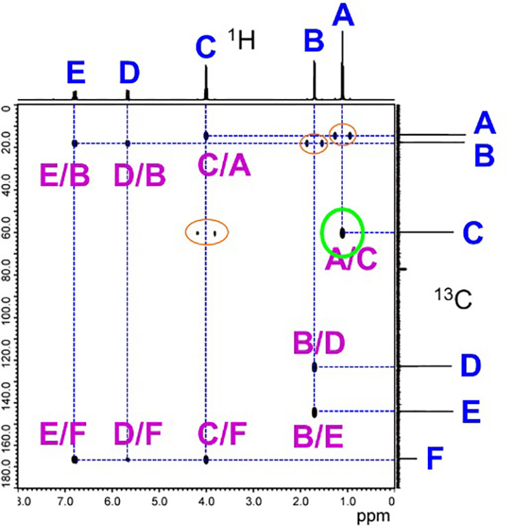
Fig. 10 HMBC Spectra
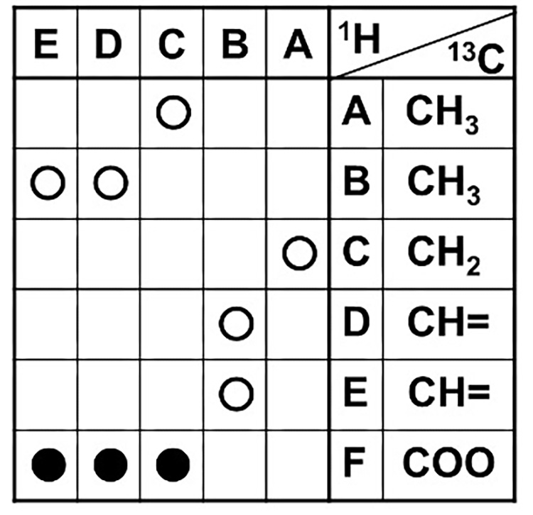
Table 6 is the correlation table for HMBC. We write the symbol for the 1H signal horizontally and the symbol for the 13C signal vertically, as per the spectrum. (Note that the symbols for the 1H signals are not necessarily in alphabetical order.) Correlation signals for the HMBC spectra will be filled in. For example, if the correlation signal is 13C for C and 1H for A, mark the intersection of C for 13C and A for 1H in the correlation table. In this way, all correlation signals are entered in the HMBC correlation table.
Table 6 HMBC Correlation Table
We use the information in the HMBC to connect the substructures.
Look at the HMBC correlation table (Table 7) that you filled out earlier. In the correlation signal marks, bonds that have already been analyzed by COSY in Step 3 are marked with ○, and bonds that were found for the first time in HMBC are marked with ●. The bond that was found for the first time in HMBC is the COO correlation for F. This indicates that F is a long-range spin couplings with C, D, and E.
Table 7 HMBC Correlation Table (2)
We will look at the long-range correlations of F-C, F-D, and F-E to consider which direction is correct for the COO to be attached, among the inferred structures I and II. (Figure 11)
First, in inferred structure I, F's 13C and C's 1H have three bonds "3JCH", ; F's 13C andD's 1H have two bonds "2JCH", ; and F's 13C and E's 1H have three bonds "3JCH".
Next, let us look at the inferred structure II. The 1H of 13C and C in F is "2JCH" with two bonds, the 1H of 13C and D in F is "3JCH" with three bonds, and the 1H of 13C and E in F is "4JCH" with four bonds.
Since 4JCH is not likely to be observed, we can expect that the inferred structure I is a reasonable structure.
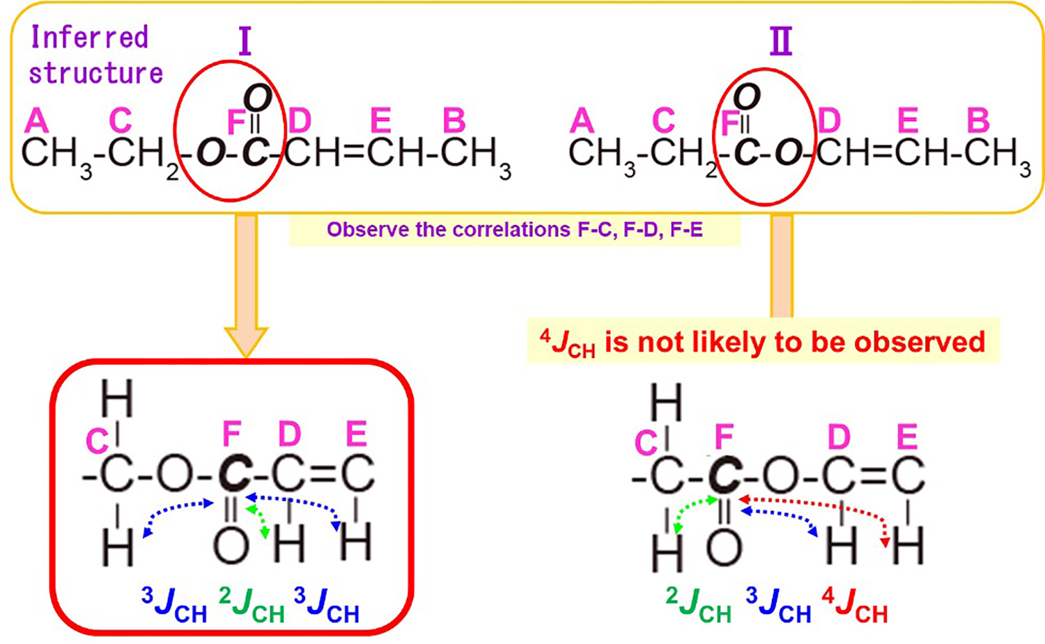
Fig. 11 Comparison between Inferred Structures I and II
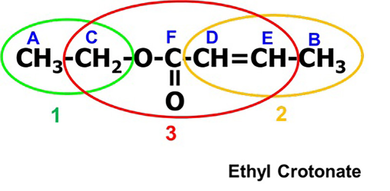
Finally, the inferred structure I is checked against the information in the 1D-NMR spectrum of 13C to confirm if it is really correct. In the inferred structure I, CH2 of the symbol C is bonded to oxygen. And the 13C chemical shift of this C was 59.8 ppm (Table 1).
The 13C chemical shift table for CH2 (Table 8) shows that normal CH2 is observed at 20-45 ppm, while CH2 bonded to oxygen is observed at 40-70 ppm with a lower field shift.
From this fact, we can conclude that "Structure I is correct".
Table 8 13C Chemical Shift for CH2
| Chemical Shift | |
|---|---|
| - CH2 - | 20 -45 ppm |
| - CH2O - | 40 - 70 ppm |
Related Applications
Need for high resolution 2D spectra
NOAH-NMR Supersequences with Nested Acquisition for Small Molecules
Application of DOSY: Analysis of guest encapsulation
Observation of NOE by HSQC-NOESY
Products
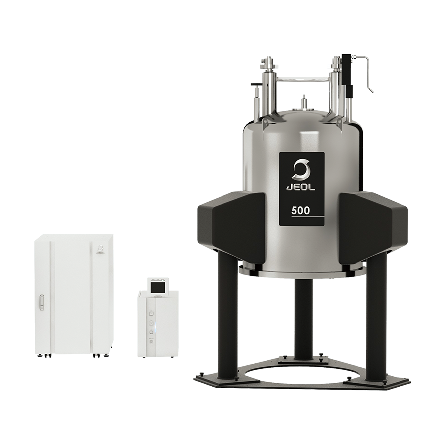
Nuclear Magnetic Resonance Spectrometer (NMR)
NMR is the abbreviation for Nuclear Magnetic Resonance. It is an instrument used to observe the resonance phenomenon of nuclear spins by placing atomic nuclei in the magnetic field to analyze molecular structure of a substance at an atomic level. Specifically, it is useful in the analysis of organic compounds and polymer materials and used in the fields of pharmaceutical, biology, food, and chemistry. The application is even recently expanding to include the analysis of structural and physical properties of inorganic materials such as ceramics and batteries.
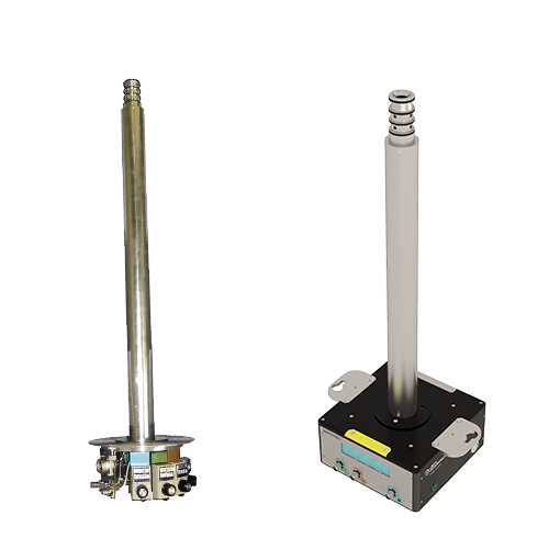
NMR Probes
With NMRs, the detector (probe) differs depending on the sample form and measurement technique. JEOL offers solution and solid probes for a wide variety of purposes.
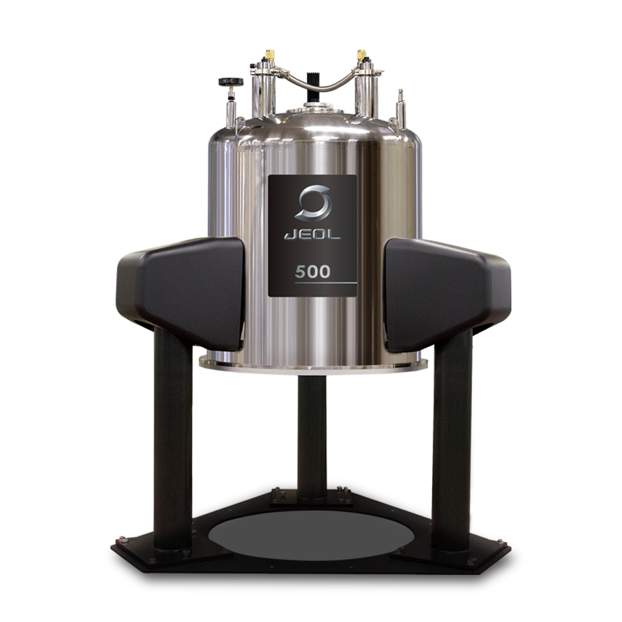
Superconducting magnets (SCM)
Space-saving design with a compact superconducting magnet. Greater flexibility of installation layout of the instrument is possible with the new compact magnets that have a smaller stray magnetic field.
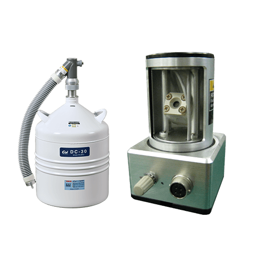
NMR Peripheral Equipment
Introducing NMR peripherals such as the Auto Sample Changer and Nitrogen Replenishment System.

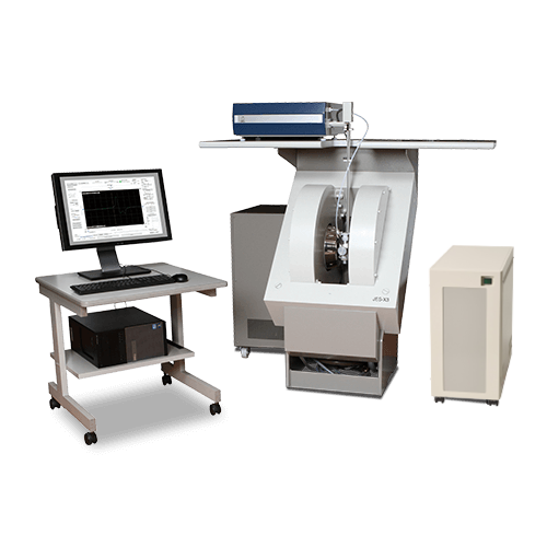
Electron Spin Resonance Spectrometer (ESR)
Electron Spin Resonance (ESR) is a powerful analytical method to detect, analyze and determine thecharacteristics of unpaired electrons in a substance. It is clear that the state of electrons in a substance have a strong influence on its characteristics and functionality, so evaluation by ESR is becoming more and more important. Many types of substances, from electronic materials to catalysts, biological samples, can be studied regardless of whether they are solid, liquid, or gas. A wide range of ESR techniques are possible using suitable attachments together with the basic instrument.
JEOL Ltd.
Since its foundation in 1949, JEOL has been committed to the development
of cutting-edge scientific and metrology instruments, industrial and medical equipment.
Today,
many of our products are used throughout the world and we are highly regarded as a truly global
company.
Aiming to be a 'top niche company that supports science and technology around the
world', we will continue to respond precisely to the increasingly sophisticated and diverse needs
of our customers.