Diffusion Analysis Multi — Multiple Exponential Function Fitting for PFG-NMR data —
NM220006E
Pulsed-Field Gradient Nuclear Magnetic Resonance (PFG-NMR) is utilized to analyze the self-diffusion of molecules and ions. The self-diffusion coefficient (D) in PFG-NMR is determined by recording the decay of signal intensity through a series of experiments using either Pulsed Gradient Spin Echo (PGSE) or Pulsed Gradient Stimulated Echo (PGSTE) sequences with varying gradient strengths (G). The decay of signal intensity is subsequently analyzed using curve fitting or inverse Laplace transformation methods. The Delta NMR software provides a curve analysis tool that supports the fitting of PFG-NMR data. Versions 5.3.3 and earlier of the Delta NMR software support curve fitting using a model that assumes a single self-diffusion coefficient contributing to the decay. However, starting from the Delta NMR software version 6.0 and onwards, there is support for curve fitting using the "Diffusion Analysis Multi" feature. This feature enables the analysis to account for multiple self-diffusion coefficients during the curve fitting process.
Background
The Stejskal-Tanner formula (1) describes a decay curve where a single self-diffusion coefficient contributes to the decay process [1].
 (1)
(1)
In this context, IG=0 represents the signal intensity at G=0, while γ denotes the gyromagnetic ratio. Additionally, δ refers to the duration of the PFG, and Δ* represents the corrected diffusion time, which takes into account the shape factor of the PFG [2]. The function I(G) exhibits a (half) Gaussian function with respect to G and an exponential decay with respect to G2. If the decay consists of a single self-diffusion coefficient, the self-diffusion coefficient can be determined using linear regression in formula (2). Formula (2) is obtained by taking the logarithm of both sides of formula (1). The self-diffusion coefficient (D) can be determined as the negative slope in the regression analysis, where In(I(G)/IG=0) is proportional to (γGδ)2Δ*.
 (2)
(2)
When multiple self-diffusion coefficients contribute to the signal decay in a curve, an extended multi-component model function, as defined in formula (3), is required to analyze each diffusion coefficient.
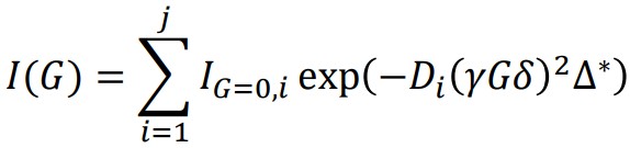 (3)
(3)
Here, j represents the number of self-diffusion coefficients contributing to the signal decay. The logarithmic transformation strategy used in formula (2) is not applicable to this multi-component model function. Hence, in formula (3), IG=0,i and Di are determined numerically through a non-linear least squares problem-solving approach. In this problem, initial values of IG=0,i and Di are necessary. It is important to note that the numerical solutions of G=0,i and Di may vary depending on the chosen initial values. The following section elucidates the procedures involved in the regression functionality of the "Diffusion Analysis Multi" mode, which has been implemented in the Delta software starting from version 6.0. The "Diffusion Analysis Multi" mode regression is specifically designed to analyze decay curves that involve multiple self-diffusion coefficients, utilizing formula (3).
Tutorial using a mixture solution of two monodispersed polystyrene samples with varying average molecular weights
In this tutorial, we will walk you through the procedures for analyzing a mixed solution of two monodispersed polystyrene samples with different average molecular weights using the "Diffusion Analysis Multi" mode in the Delta NMR software version 6.0 or later. Specifically, we will work with a mixture comprising equal amounts of two polystyrene samples: one with an average molecular weight (Mw) of 3,510 Da and a number average molecular weight (Mn) of 3,350 Da, and the other with an Mw of 35,400 Da and an Mn of 34,400 Da. The solvent used for the mixture is o-dichlorobenzene-d4, and the concentration is set at 4 wt%.
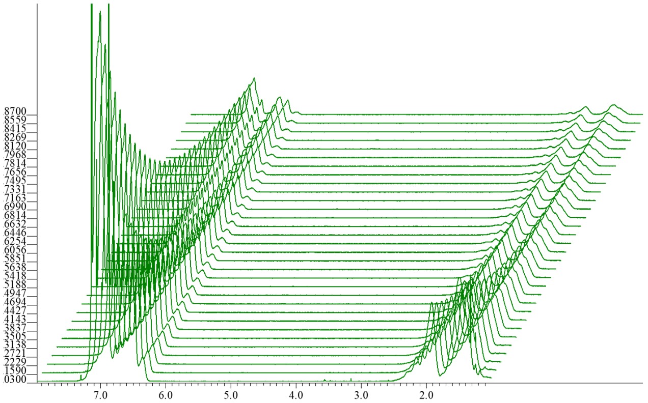
Figure 1 Decay curves obtained from a PGSTE experiment using a mixture solution of two monodispersed polystyrenes with different molecular weights (one with Mw: 3,510 Da and Mn: 3,350 Da, and the other with Mw: 35,400 Da and Mn: 34,400 Da).
After completing the NMR measurement, the initial step involves processing the x dimension in the arrayed data. Figure 1 displays the Fourier-transformed arrayed spectra. In this case, the 'stack' display mode is used. The '4' key is a shortcut for the 'stack' display mode in the Delta NMR software. Select the ‘Analyze’ option from the toolbar in the Data Slate. From the drop-down menu, choose ‘Curve Analysis’.
Activate the ‘Peak’ mode by clicking the ‘Peak’ button. Pick the peak(s) to be analyzed using the ‘Peak’ mode button or ‘Peak Pick’ button, then select the picked peak(s). Select the ‘Diffusion Analysis Multi’ mode from the pull-down menu in the Curve Analysis tool. When you press the 'Apply' button with the current settings, the fitting process is performed using a single model (Formula 3 with j=1). In this case, our objective is to fit the data to a model with two self-diffusion coefficients (Formula 3 with j=2). To incorporate these additional parameters, you can press the ‘Add parameter’ button. After pressing the ‘Add parameter’ button, four fields [1] D, [1] I(0), [2] D, and [2] I(0) are displayed, as shown in Figure 2. The values [1] D, [1] I(0), [2] D, and [2] I(0) correspond to the self-diffusion coefficient of the 1st component, the signal intensity at G=0 of the 1st component, the self-diffusion coefficient of the 2nd component, and the intensity at G=0 of the 2nd component, respectively. To initiate the calculation, you need to set the initial values*,** in each respective field. Once you have set these values, press the ‘Apply’ button to perform the calculation. (Remark: In the one-component analysis, the results serve as a reference for the initial estimation. Unlike the multi-component analysis, the single-component analysis does not require manual input of initial values, as these values are determined internally.)
* In this context, please set the numerical value only (which should be other than 1) for each field. It's important to note that the diffusion coefficient should be specified in [m²/s] and not in [cm²/s].
** Notation with powers of ten (e.g., 9.9e-10) is acceptable. However, it is important to include the number of the first decimal place (e.g., 1.0e-11 is acceptable, while 1e-11 is not).
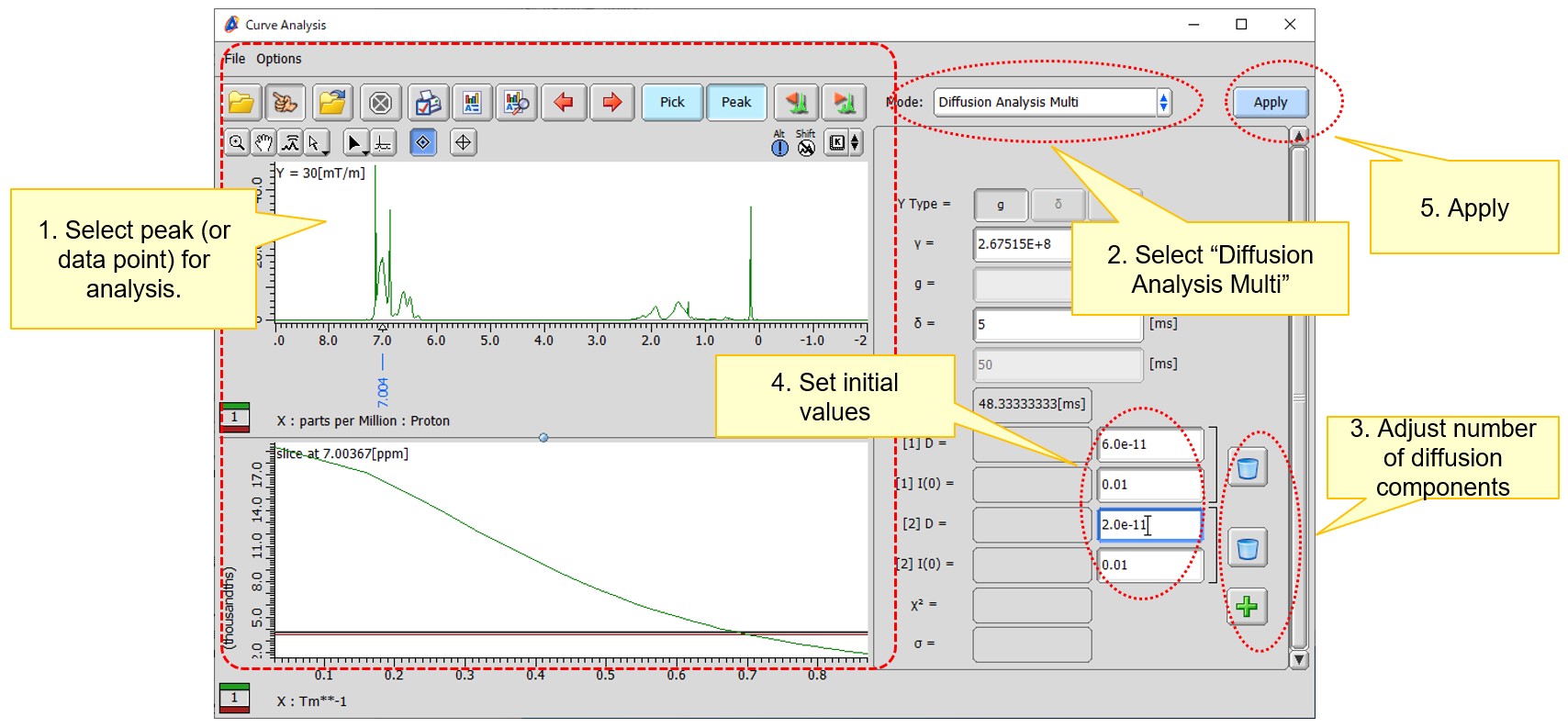
Figure 2 Steps involved in multi-component fitting of a decay curve in the ‘Diffusion Analysis Multi’ mode.
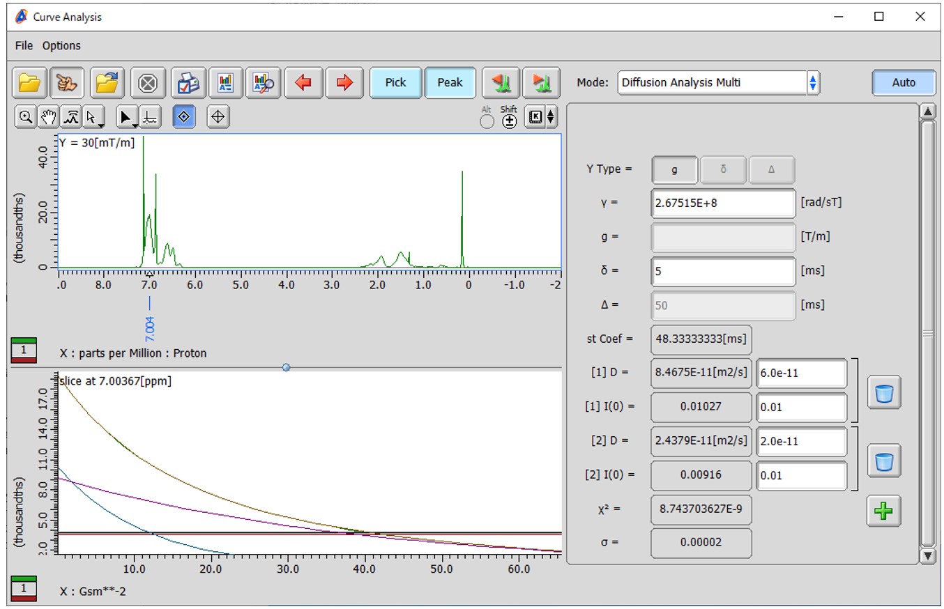
Figure 3 Result of fitting to a two-diffusion coefficient model using a decay curve obtained from a PGSTE experiment on a mixture solution of two polystyrene samples with different molecular weights (one with Mw: 3,510 Da and Mn: 3,350 Da, and the other with Mw: 35,400 Da and Mn: 34,400 Da).
The results of the “Diffusion Analysis Multi” mode are shown in Figure 3. In this case, the analysis was conducted using a decay curve obtained at 7.00 ppm, specifically from the aromatic proton, in the PGSTE experiment of the mixed solution of monodispersed polystyrenes. The initial values for the parameters [1] D, [1] I(0), [2] D, and [2] I(0) were set to 6.0e-11, 0.01, 2.0e-11, and 0.01, respectively. The analysis estimated that the curve consisted of a self-diffusion coefficient of 8.47e-11 m²/s for one component and 2.44e-11 m²/s for another component. The initial intensities for these components were estimated to be 0.0103 and 0.0092, respectively. These values were obtained as part of the analysis in the "Diffusion Analysis Multi" mode. Additionally, the Chi-square value (χ2) and the standard deviation (σ) are provided as indicators of the residuals between the experimental decay curve and the fitted model. These values help assess the goodness of fit and the accuracy of the model in representing the observed data. In the lower-left panel, the horizontal axis represents (γδG)2, which corresponds to the decay behavior of the components in the analysis. Each component decays exponentially in this plot. The plot serves as a visual representation of the fit quality. The plot consists of multiple layers. The first layer (default color: green) represents the experimental data, while the second layer (default color: brown) represents the fitted model, which is the sum of all components. From the third layer onwards (blue and purple), each layer represents the exponential decay of each diffusion component. This layered visualization helps distinguish and assess the contributions of each component to the overall decay behavior.
Remark: It is important to note that the analysis in the ‘Diffusion Analysis Multi’ mode can sometimes encounter local minima, particularly if the initial estimates are not accurate. Since the results obtained in this mode are numerical solutions, they can be sensitive to the initial values provided. Additionally, numerical solutions can be unstable, especially when the noise in the decay curve is significant and when the diffusion coefficients are close in value. In multi-component fitting problems, increasing the number of components generally leads to a smaller residual in the fit. However, it is crucial to understand that this does not necessarily mean that the number of components in the model corresponds to the actual number of diffusion components in the system being analyzed. It is important to carefully consider the appropriate number of components for the analysis based on the specific system and experimental data. Taking these factors into account, it is recommended to conduct the analysis with careful consideration of the initial estimates, noise levels, and the appropriate number of components to achieve reliable and meaningful results.
References
[1] Stejskal, E.O., Tanner, J.E., “Spin diffusion measurements: Spin echoes in the presence of a time-dependent field gradient”, J. Chem. Phys., 42 (1965) 288-292.
[2] Sinnaeve, D., “The Stejskal–Tanner Equation Generalized for Any Gradient Shape—An Overview of Most Pulse Sequences Measuring Free Diffusion”, Concept. Magn. Reson., 40A (2012) 39-65.
Solutions by field
Related products
Are you a medical professional or personnel engaged in medical care?
No
Please be reminded that these pages are not intended to provide the general public with information about the products.