Chemometric Tool — Gateway to Chemometrics with NMR Data —

Chemometrics is a discipline that utilizes data mining techniques, including dimensionality reduction, discrimination, visualization, and regression, to extract information from extensive sets of experimental analytical data. NMR spectroscopy, a highly quantitative and reproducible technique, allows for non-invasive analysis of chemical species with minimal sample preparation. This is particularly advantageous for data mining, as NMR spectra, including series of 1H NMR spectra of biological samples, are commonly employed as input for multivariate analysis. The Chemometrics tool has been incorporated into the Delta NMR software since version 6.0. It facilitates exploratory multivariate analysis by converting series of 1D NMR spectra into a matrix. The 'Chemospec' package [1] in the R language for statistical computing serves as the engine for multivariate analysis. When the 'Chemospec' package is installed, the Delta software offers a seamless user interface for exploratory multivariate analysis.
The Chemometrics tool initially converts multiple NMR spectra into a multidimensional matrix, with dimensions suitable for data mining using bucket integration. Additionally, the Chemometrics tool offers support for exploratory multivariate analyses, such as Principal Component Analysis (PCA) and Hierarchical Cluster Analysis (HCA) with an optional heat map display. These methods do not require labeled training data. However, it does not provide support for other data mining techniques such as discrimination analysis and regression analysis. On the other hand, the R language offers a wide range of data mining techniques through packages developed by users and developers worldwide.

Importing NMR data and preparing the input matrix for data mining through bucket integration

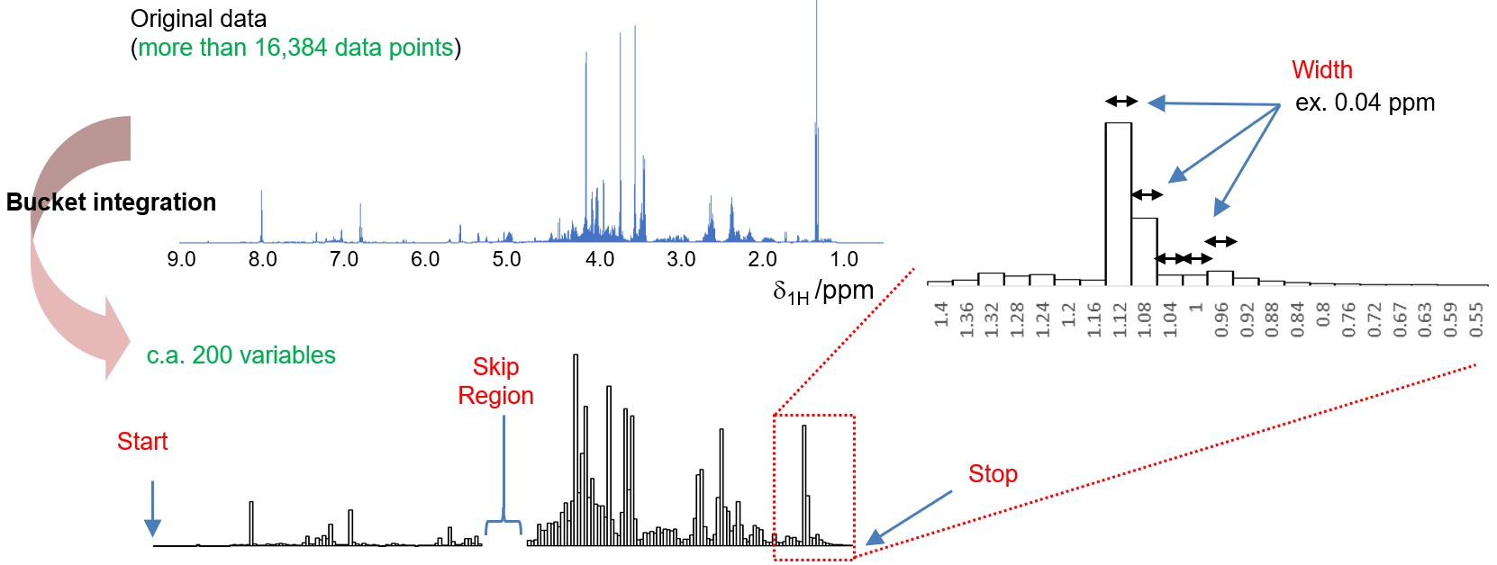
In an exploratory data analysis workflow, a series of 1D NMR data is transformed into a matrix with an appropriate number of dimensions (number of variables), and data mining techniques such as multivariate analysis are then applied to the matrix (Figure 1). Bucket integration is one of the simplest methods for generating a matrix from spectra. In the bucket integration approach, spectra are divided into equally spaced spectral windows (e.g., 0.04 ppm), and the area within each window is calculated to represent the original spectrum and used as the variable (Figure 2(a)). These windows, often referred to as 'buckets' or 'bins', contribute to the process known as bucket integration, also called 'bucketing' or 'binning'. Bucket integration effectively reduces the dimensionality from tens of thousands to hundreds. This reduction is particularly advantageous when the integrating variables are highly correlated to some extent and is robust against unwanted linewidth variations caused by an inhomogeneous magnetic field or chemical shift variations due to factors such as pH, concentration, and ionic strength, among others. However, the Delta software does not support local spectral alignment and non-uniform window bucket integration.

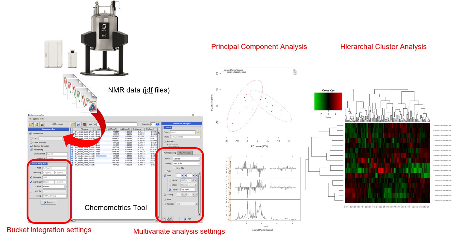
Figure 1 Schematic representations of the Chemometrics tool in Delta NMR software since version 6.0

(a)

(b)

(c)

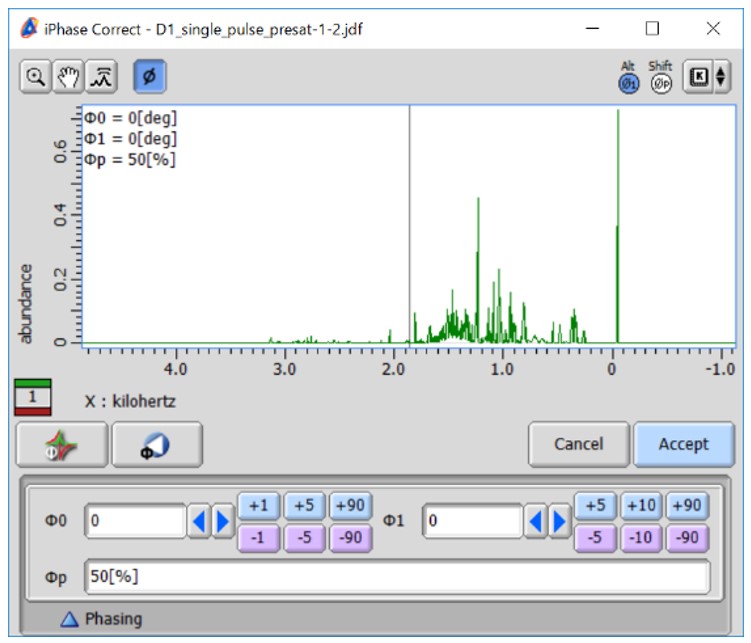
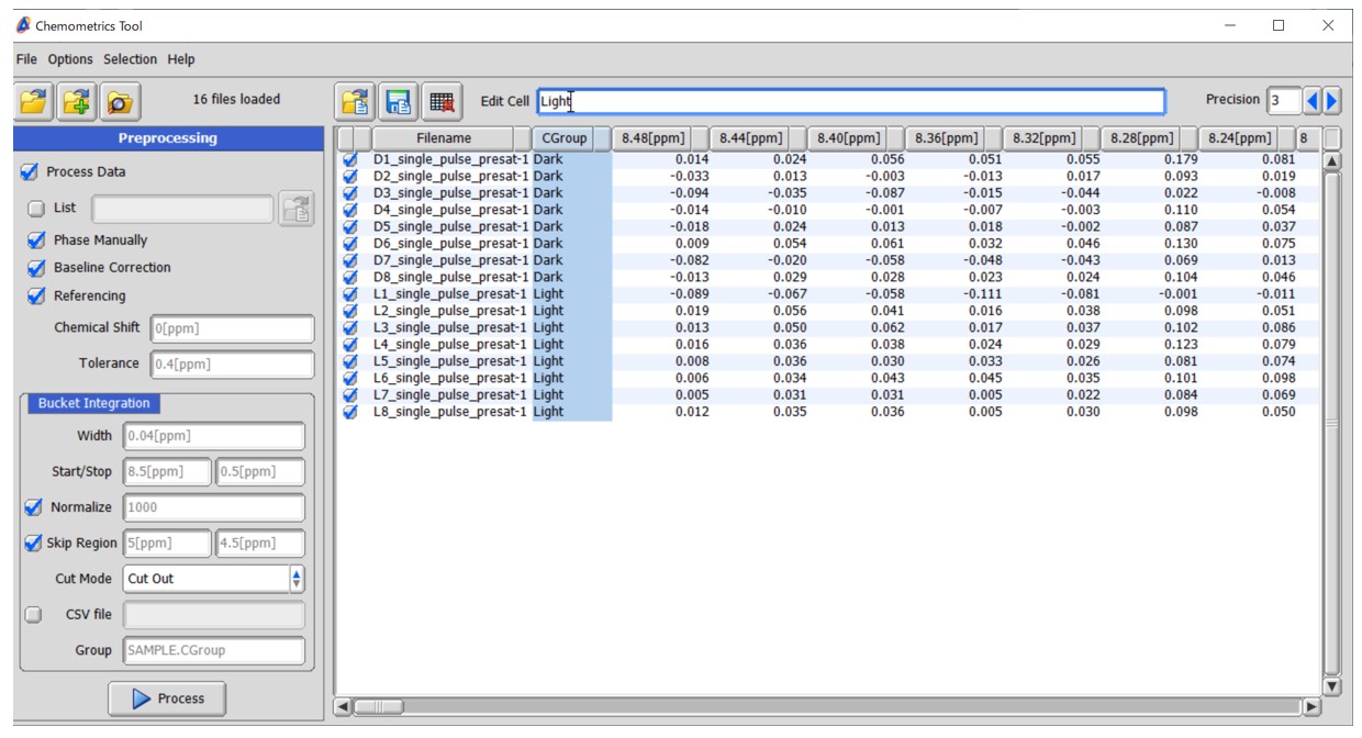
Figure 2 Bucket integration in the Chemometrics tool within the Delta NMR software version 6.0 and onwards. (a) Graphical representation of bucket integration, (b) the graphical user interface of the Chemometrics tool, and (c) The window for manual phase correction.

The user interface for setting bucket integration in the Chemometrics tool is depicted in Figure 2(b). The tool supports both unprocessed data in the time domain and processed spectra in the frequency domain. When loading unprocessed data and selecting the 'Process Data' option, the Chemometrics tool performs Fourier transform, automatic phase correction, and subsequently applies bucket integration. When the 'Phase Manually' option is checked, the Chemometrics tool allows for one-by-one manual phase correction, as depicted in Figure 2(c). When the 'Baseline Correction' option is selected, the Chemometrics tool performs 1st order baseline correction using the 'dc_correct' function. When the 'Referencing' option is selected, the Chemometrics tool performs chemical shift correction based on the 'Chemical Shift' and 'Tolerance' fields. For instance, if you set the ‘Chemical Shift’ field as 0.0 ppm and the ‘Tolerance’ field as 0.4 ppm, the Chemometrics tool will reference the highest digital point within the range of -0.2 to 0.2 ppm to 0.0 ppm. This referencing correction is particularly effective for 1H-NMR spectra that include DSS-d6 or TSP-d4 as an internal reference.
Next, let's explore the bin integration settings. To set the width of each bin, you can input the desired value in the ‘Width’ field. A commonly used range for the width of each bin is between 0.01 and 0.04 ppm [2]. To define the range of bucket integration, you can specify the desired start and stop values in the ‘Start/Stop’ fields. If the ‘Normalized’ option is selected and an arbitrary value for the total sum is set, each row, which corresponds to a spectrum, is normalized by the sum of the bins. The ‘Skip Region’ option allows you to exclude a specific region from the analysis. For instance, you can use the ‘Skip Region’ option to exclude the region containing residual signals caused by water suppression. By pressing the ‘Process’ button, the results of the bucket integration are displayed in the data window.
Here is a tutorial analysis utilizing the Chemometrics tool, based on the data from the previous application note NM170021: Supervised Multivariate and Univariate Analyses for NMR-based Metabolic Profiling to Explore Characteristic Metabolites among Sample Groups　(https://www.jeol.co.jp/en/applications/detail/1634.html). The dataset consisted of sixteen 1H NMR spectra of polar metabolites extracted from broccoli sprouts cultivated under different environments, specifically in light and dark conditions, with eight biological replicates for each condition. The Chemometrics tool utilized the following options: 'Process Data', 'Phase Manually', 'Baseline Correction', and 'Referencing (0.0[ppm], 0.4[ppm])'. The 'Skip Region' option was enabled with the Start set as 5.0[ppm] and the Stop set as 4.5[ppm]. We used the default settings for other parameters, namely ‘Width’ (0.04 ppm), ‘Start/Stop’ (8.5[ppm] and 0.5[ppm]), and ‘Normalize’ (1000). Immediately after the start of the analysis, a new window for manual phase correction of the first dataset was opened (Figure 2(c)). After correcting the phase of the first spectrum, the 'Accept' button was pressed, and the second spectrum appeared. This process was repeated for each spectrum included in the analysis. Finally, the results of the bucket integration were displayed.

Exploring Data Analysis with the “Chemospec” Package

The Chemometrics tool offers a user-friendly interface for conducting Principal Component Analysis (PCA) and Hierarchical Cluster Analysis (HCA), both with and without a heatmap. These analyses are performed using the Chemospec package in the R statistical computing language environment, which needs to be installed separately. In order to input sample category information, you can use specific letters in the second column (CGroup) of the previously generated matrix. It's important to note that PCA and HCA are unsupervised analysis techniques, which means that the sample category information is not utilized during the analysis itself. However, this information can be employed for visualizing the results effectively, such as by coloring plots based on sample categories.
PCA is a dimensionality reduction technique that summarizes information in multivariate data (original data) into much smaller dimensional space. PCA projects a large number of correlated variables into a new variable (new variables are called principal components: PCs) that can be represented by a linear combination of the original variable. In this projection, the projection coefficients are chosen to maximize the variance of the first PC (PC1) and to make the subsequent PCs orthogonal to the previously determined PCs and to maximize their variance. As a result, most of the data can be summarized in a small number of dimensions (small number of PCs). Here, the coordinates of the PCs are called the score, and the unit vector corresponding to the projection coefficients is called the loading.
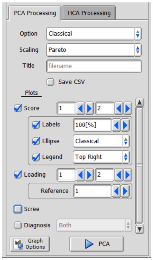
Here, Figure 3(a) illustrates the step-by-step procedure of PCA using the Chemometrics tool in the Delta NMR software. Both the 'Classical' and 'Robust' versions of PCA can be accessed from the 'Option' menu in the "PCA processing" tray of the Chemometrics tool. The 'Classical' option refers to the common PCA method that assumes data normality, while the 'Robust' option refers to the robust version of PCA that does not assume data normality. The 'Classical' PCA utilizes the arithmetic mean and variance as indicators of central tendency and variability, respectively. In contrast, the 'Robust' PCA utilizes the L1-median and the square of the median absolute error (MAD) instead of the arithmetic mean and variance. The 'Robust' PCA is known for its reduced sensitivity to outliers. When using the 'Classical' PCA, you can choose a scaling method from options such as 'Auto' (auto scaling), 'Pareto' (Pareto scaling), and 'No Scale' (only centering is performed) in the ‘Scaling’ menu. When you check the 'Score' menu in the Chemometrics tool, it generates a score plot between two specified principal components (Figure 3(b)). When you check the 'Loading' menu in the Chemometrics tool, it generates a loading plot between two specified principal components (Figure 3(c)). The Chemometrics tool provides additional diagnostic tools for identifying outliers, including a scree plot displaying the percentage of accumulated variance, a score distance plot, and an orthogonal distance plot. These plots can be used to assess the presence of outliers in the data. For more detailed information on the Chemometrics tool and its usage, please refer to Chapter 7 titled 'Liquid Application User’s Manual' in the user's manual for the JNM-ECZ/ECZL series.
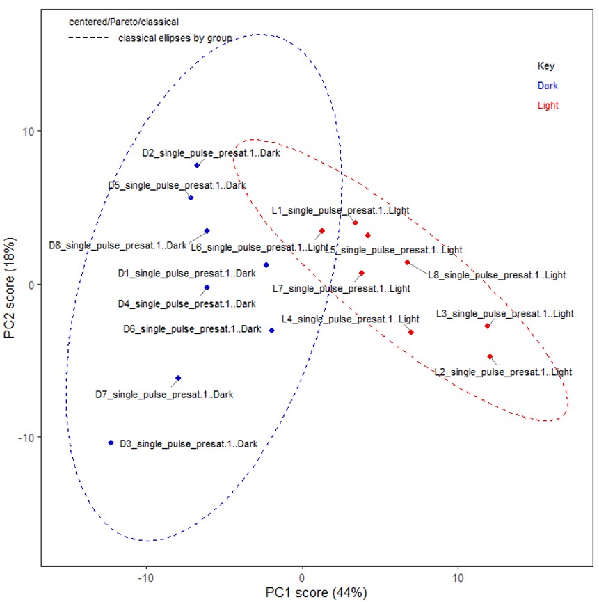
In the tutorial, the sample category information was pre-defined as ‘Dark’ and ‘Light’ in the second column (as shown in Figure 2(b)). Then, for the analysis, the 'Classical' and 'Pareto' options were selected in the Chemometrics tool. The 'Score' and 'Loading' boxes in the Chemometrics tool were checked, and the first two principal components (PC1 and PC2) were selected for visualization and analysis. Subsequently, PCA was performed using the selected options and variables. In the tutorial, the score plot (PC1 vs PC2) clearly exhibited a distinct separation between the sample categories. PC1 demonstrated a strong association with the variations in the sample categories, effectively capturing the main source of variance in the dataset. The scores in the PCA are obtained as a linear combination of the original variables, capturing the variations present in the dataset. On the other hand, the loadings correspond to the projection coefficients that determine the contribution of each original variable to the construction of the PCs. Indeed, in the context of PC1, the negative loadings for certain metabolites suggest that these metabolites are more abundant in dark-grown broccoli sprouts. This is supported by the negative scores observed for these samples in PC1 (Figure 3(c)). The relationship between the loadings and scores in PC1 indicates that the variations in these specific metabolites strongly contribute to the separation of samples based on their growth conditions. By analyzing the scores and loadings in this manner, we can identify metabolites that exhibit significant differences between sample groups and gain insights into the underlying factors driving these differences.

(a)

(b)

(c)

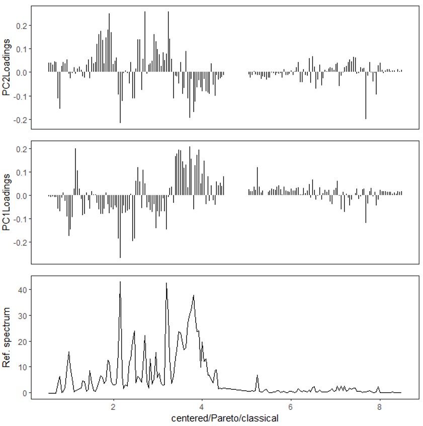
Figure 3 PCA in the Chemometrics tool in the Delta NMR software version 6.0 and onwards. (a) User interface, (b) a score plot (PC1 vs PC2) of classical PCA, and (c) a loading plot.

HCA is an unsupervised multivariate analysis technique that is commonly used for exploring patterns and relationships within multivariate datasets. It is particularly useful for identifying clusters or groups of samples with similar variate patterns. HCA generates a dendrogram, which is a tree-like structure, based on the distance or dissimilarity between samples calculated from the multivariate data. The dendrogram visually represents the hierarchical relationship between samples, showing how they cluster together based on their similarities or differences. In addition to the dendrogram, HCA can also be used to generate a heatmap. The heatmap provides a visual representation of the distribution of each metabolite in the clusters of each sample. It rearranges the rows and columns based on the results of the HCA, placing similar samples and metabolites closer together. This allows for the identification of patterns and trends in the dataset, highlighting metabolites that show similar behavior across certain sample clusters.
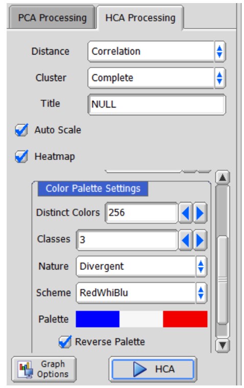
Here, the procedures of HCA in the Chemometrics tool are depicted in Figure 4(b). Distance in HCA is defined in the ‘Distance’ menu. Eleven distance indicators are available in the pull-down menu. Clustering methods, which define the distance between ‘cluster and object’ or ‘cluster and cluster’ are defined in the ‘Cluster’ menu. For detailed information about distance and clustering methods, please refer to Chapter 7 titled 'Liquid Application User’s Manual' in the JNM-ECZ/ECZL series user’s manual. A heatmap is generated when the ‘Heatmap’ option is enabled. The heatmap visualizes the distribution of each metabolite within clusters of each sample by rearranging the rows and columns based on HCA performed separately for samples and variables. When the ‘Heatmap’ option is set to false, sample-wise HCA is performed. This means that the clustering is based on the similarity between samples, and the rows of the heatmap are rearranged accordingly. The color settings in the ‘Color Palette Setting’ determine the color scheme used in the heatmap. If the ‘Heatmap’ option is set to true, pressing the ‘HCA’ button in the Chemometrics tool will immediately display the heatmap in a new window.
In the tutorial, the "Correlation" option was selected for calculating the distance. The correlation distance is a dissimilarity measure that is based on the Pearson's correlation coefficient. The ‘Complete’ clustering method was used. The variables were auto-scaled using the 'Auto Scale' option, and the 'Heatmap' option was selected to generate a heatmap. The generated heatmap is depicted in Figure 4(b). The ‘dark’ and ‘light’ groups are observed to form distinct clusters on the sample-wise HCA dendrogram, as shown on the left side of the heatmap. Based on the heatmap, it can be observed that the ‘Dark’ group exhibits higher abundance of amino acids, whereas the ‘light’ group shows higher abundance of saccharides.

(a)

(b)

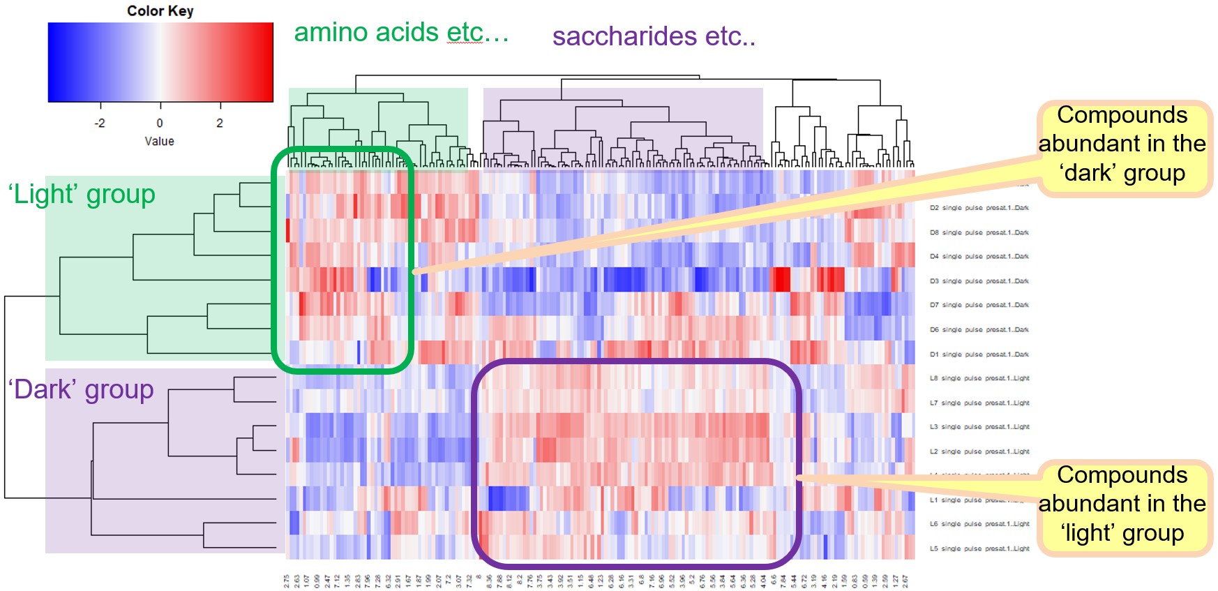
Figure 4 HCA in the Chemometrics tool in the Delta NMR software version 6.0 and onwards. (a) User interface, and (b) a heatmap whose rows and columns have been rearranged by the sample-wise and variable-wise HCA, respectively.

How to set up the Chemometrics tool in the Delta NMR software

To perform PCA and HCA on the Chemometrics tool interface, install the R environment along with the Chemospec package and its related packages. Set the file path of the Rscript.exe executable to the ‘Rscript Executable’ parameter in the External tab of the preferences in the Delta NMR software. For detailed instructions on the configuration and preparation of the Chemospec package, refer to Chapter 7.2 titled ‘Configuration and preparation of Chemospec package’ in the 'Liquid Application User's Manual' of the JNM-ECZ/ECZL series user's manual.

Reference

[1] B.A. Hanson (2021). ChemoSpec: Exploratory Chemometrics for Spectroscopy. R package version 5.3.21. https://CRAN.R-project.org/package=ChemoSpec, [2] A.H. Emwas, E. Saccenti, X Gao,R.T. McKay, V.A.P. Martins dos Santos, R. Roy, D.S. Wishart, Metabolomics (2018) 14:31, [3] C. Croux, P. Filzmoser, and M.R. Oliveira, Chemometr Intell Lab Syst. 87 (2007) 218-225.

Solutions by field

Battery

Energy

Chemistry

Plastics / Polymer

Laboratory / Pathology

Biology / Life science

Medicine

Food / Plant

Environment

Others

Related products

JNM-ECZL series FT NMR