2D homonuclear correlation 1H solid-state NMR by wPMLG
NM200011E
Multidimensional correlation NMR spectroscopies, which provides inter-nuclear proximity/connectivity, play a crucial role to probe the atomic resolution structures. Especially, 1H-1H homonuclear correlation spectroscopy is quite useful source of information because of high abundance (>99%) and gyromagnetic ratio, thus resulting in strong inter nuclear interactions. Thanks to the development of high resolution 1H solid-state NMR, now it is feasible to observe 1H-1H correlation high resolution solid-state NMR [1]. There are two distinctive categories; 1) single quantum (SQ)/SQ correlation and 2) double quantum (DQ)/SQ correlations. In this note we introduce 2D 1H SQ/ 1H SQ and 1H DQ/ 1H SQ correlation spectroscopy to probe the internuclear proximity using high-resolution 1H solid-state NMR techniques.
1H SQ/ 1H SQ correlations
SQ coherence is observed in the indirect t1 dimension, thus essentially the same spectra appear in both dimensions. This makes spectral interpretation straightforward. The connectivity can be read from the off-diagonal cross peaks. The sequence is essentially the same as NOESY experiments, but wPMLG is applied during the t1 and t2 dimensions to achieve 1H-1H decoupling during spin evolution (Fig 1). The first pulse excites the SQ coherence. Followed by the t1 evolution, the magnetization is stored along the z-axis by the second 90 degree pulse. The 1H magnetization is diffused to the other 1Hs during the mixing time. Finally, the magnetization is observed during t2 after third 90 degree pulse. In this approach, 1H-1H correlation is established during the mixing time between the indirect SQ and direct SQ dimensions. As the magnetization stored along the z-axis, one can elongate mixing time to the order of 1H T1, allowing multiple relayed coherence transfer, or spin diffusion. Thus, SQ/SQ can potentially provide long range (~100 A) correlations. In addition, the semi-quantitative distance measurement can be achieved by monitoring of build up of correlation peaks. Typically the build up curve is evaluated with empirical spin diffusion equation [2], however, explicit spin dynamic calculation can also be applied [3]. One drawback is presence of uncorrelated peak on the diagonal line. This hampers the observation of correlations between the nuclei possessing identical or very close chemical shifts.
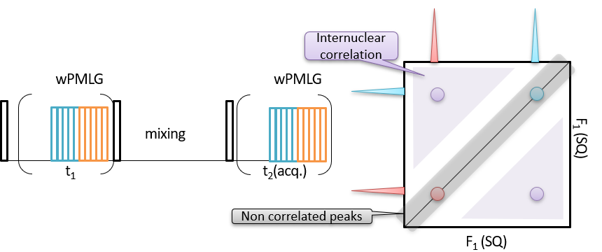
Fig 1.
Pulse sequence (left) and schematic representation of 1H SQ/1H SQ correlation spectrum (right).
1H SQ/ 1H SQ correlations: experimental setup
wPMLG decoupling is optimized by spin echo experiments. We recommend z-rotation wPMLG supercycling to avoid the necessity of trim pulses. As no acquisition window is required in the indirect dimension, windowless PMLG or the other windowless 1H-1H decoupling sequences can be used during t1. However, this introduces different scaling factor in the t1 dimension than that in t2, complicating processing. Here we recommend to use the same 1H decoupling sequence as the t2 dimension for the sake of simplicity. The indirect spectral width is automatically synchronized to the wPMLG block, and defined by LG_Loop in the pulse program. The signal is sampled every LG_Loop times of wPMLG block in the indirect dimension. By maximizing LG_LOOP or minimizing indirect spectral width, one can reduce the experimental time. One can easily optimize the minimum indirect spectral width by investigating the 1D wPMLG spectrum. As 1D wPMLG spectrum is sampled every wPMLG block, the spectral width is automatically set as 1/cycle_time. Thus the spectral range is from -1/(2 x cycle_time) to +1/(2 x cycle_time). If the peaks appear only between -1/(n x 2 x cycle_time) to +1/(n x 2 x cycle_time), one can safely sample signal every n x cycle time of wPMLG. As shown in Fig 2, LG_LOOP = 4 is wide enough to cover the spectral range in this case. However, the artifacts which appear in the outside the peak area will be folded into the spectral range by setting LG_LOOP larger than one.Thus, if time allows, LG_LOOP = 1 is preferable to avoid complexity. Since 1H-1H spin diffusion is rapid enough at moderate MAS rate, no rf field is applied during the mixing time in most cases. However, recoupling/decoupling sequence can be applied if needed [4]. As the mixing time works as z-filter, or in other words, residual transversal magnetization is suppressed during the mixing time, 2 step phase cycling is enough for coherence pathway selection. In case of zero or very short mixing time, additional 3 step phase cycling, which makes the total 6-step phase cycling, is needed to suppress transversal magnetization during the mixing time. While long mixing time can be used to diffuse 1H magnetization to remote 1Hs, the mixing time has to be shorter than 1H T1. Otherwise the signal will be lost.
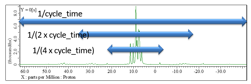
Fig 2.
1H wPMLG spectrum of L-tyrosine.HCl at 12 kHz under 14.1 T. The spectral width is automatically set to 1/cycle_time. As all the peak apper in - 1/(4 x 2 x cycle_time) to +1/(4 x 2 x cycle_time), the sampling every four cycle time of wPMLG is enough to cover all the spectral area in the indirect dimension of 1H SQ/1H SQ correlation spectra.
1H SQ/ 1H SQ correlations: data processing
The direct dimension is the same as 1D wPMLG. Linear_Ref and Reference should be applied to correct chemical shift scalings. As the indirect dimension represents SQ chemical shift, the same scaling can be applied. Fig 3 shows the resultant 2D spectrum and process list used.
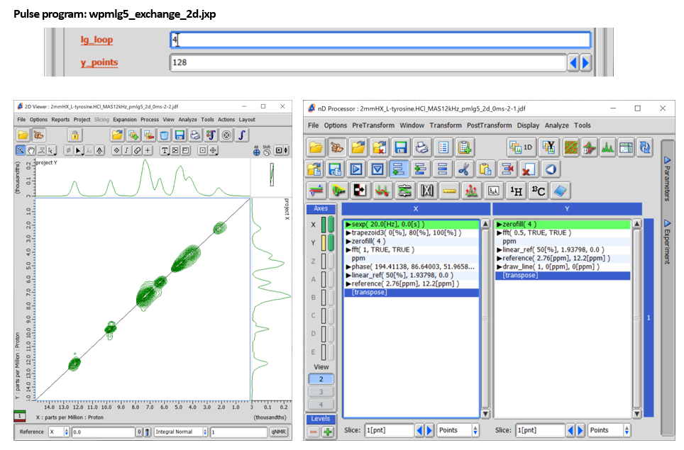
Fig 3.
1H SQ/1H SQ correlation spectrum of L-tyrosine.HCl at 12 kHz under 14.1 T (left). wPMLG decoupling is applied to both t1 and t2 dimensions. No mixing time is used (mixing time = 0). The process list is basically the same as regular 2D but Linear_Ref and Reference function should be applied to the both dimension (right). The increment of the indirect dimension is set to four times of the wPMLG cycle time by putting Lg_loop = 4. 128 t1 points were collected with 6 cans for each. The total measurement time was 128 x 6 x 2 x 1.5 s (repetition delay) = 39 mins.
No correlation peaks appear in Fig 3, because of devoid of mixing time. However, even very short mixing time of 50 us introduces cross peaks between neighboring 1Hs (Fig 4a). The intensities of cross peaks rapidly grow as the mixing time. (Fig 4b and c). The analysis of build up provides semi-quantitative distance information between 1Hs.
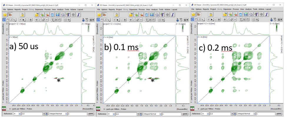
Fig 4.
1H SQ/1H SQ correlation spectrum of L-tyrosine.HCl at 12 kHz under 14.1 T at a mixing time of 50 us (a), 0.1 ms (b) and 0.2 ms (c). The glitch marked asterisk is artifact appearing at the center of the indirect dimension. The increment of the indirect dimension is set to four times of the wPMLG cycle time by putting Lg_loop = 4. 128 t1 points were collected with 2 cans for each. The total measurement time was 128 x 2 x 2 x 1.5 s (repetition delay) = 13 mins for each.
1H DQ/ 1H SQ correlations
Proximity between 1Hs can be monitored by 1H DQ/1H SQ correlation spectroscopy as well (Fig 5). Unlike 1H SQ/1H SQ correlation, 1H DQ/1H SQ correlation gives very local proximity below < 4A, and is useful to probe the atomic resolution structure. In this experiments, first DQ coherence is created by the DQ excitation block. The DQ coherence is evolved during t1 period under wPMLG irradiation. Then it is converted to longitudinal magnetization by the DQ reconversion block. A shoft z-filter could be inserted before the final read 90 degree pulse. Finally, SQ coherence is observed under wPMLG decoupling. The close similarity to 1H SQ/1H SQ sequence can be found. In fact, DQ/SQ sequence can be described by replacing the first and second 90 degree pulse in SQ/SQ to DQ excitation and reconversion blocks, respectively. The major difference is mechanism to establish 1H-1H correlation. While SQ/SQ experiments utilize 1H-1H spin diffusion during the mixing time, the two spin DQ coherences which are created by the DQ excitation block reports the two spin proximities in DQ/SQ experiments. The dipolar truncation during the DQ recoupling hampers the creation of DQ coherence between remote spins. Thus only short (typically < 4 A) 1H proximity is observed. All the correlation appear in DQ/SQ spectra come from two spin connectivities in 4 A. No uncorrelated peaks appear. This makes spectral interpretation simple. The schematic 2D DQ/SQ spectrum is shown in Fig 5. Two peaks appear at ωA and ωB in the SQ dimension. The correlation between like spin between A and A appear at ωA +ωA = 2ωA in the indirect dimension, thus (DQ, SQ) = (2ωA , ωA ). For this reason, diagonal line is plotted with a slope of 2 passing at (0, 0) ppm. The devoid of correlation at (DQ, SQ) = (2ωA , ωA ) shows that B doesn’t have like spin in close distance. The correlation between A and B appears at (DQ, SQ) = (ωA + ωB, ωA ) and (ωA + ωB, ωB ) with equidistance from the diagonal line.
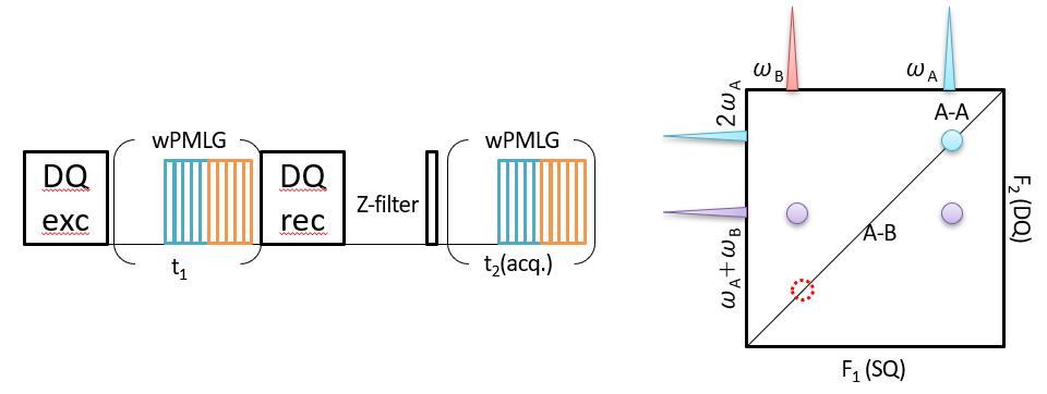
Fig 5.
Pulse sequence (left) and schematic representation of 1H DQ/1H SQ correlation spectrum (right). All the peaks appearing in the spectra are correlated peaks.
1H DQ/ 1H SQ correlations: experimental setup
The same wPMLG block with z-rotation is applied during both t1 and t2 periods. Although any 1H DQ recoupling scheme, in principle, can be used for excitation and reconversion periods, we recommend POST-C7 because of robustness to experimental imperfections and its gamma-encoded nature [5,6]. As POST-C7 require rf-field strength seven times of the MAS rate, maximum MAS rate is often limited by the 1H rf-field capability of the probe. For example, the probe which can accept 100 kHz 1H irradiation accommodates POST-C7 at 100/7 = 14.3 kHz MAS rate. Thus, MAS rate has to be carefully chosen so that POST-C7 can be applied. POST-C7 has only one parameter to be optimized, i.e. rf-field strength. The experimental optimization can be done by comparing 1D spectra at t1 = 0 with varying rf field strength (obs_amp_c7). (Fig 6) As POST-C7 is quite robust to rf field strength variation, no need to fine step tuning. We typically vary every 5 kHz or so. The DQ filtering efficiency compared to regular 1D wPMLG is typically found in 5-20% for rigid solids. It should be noted that the peaks in the indirect DQ dimension appears not at the center, but at the spinning sideband position due to DQ recoupling mechanism. [7] POST-C7 recouples m = 1 terms in the gamma-encoded manner, thus the peak appears at the +1 SSB positions, or in other words, all the peaks shifted with the MAS rate toward high frequency side (Fig 7). Thus the peak positions can be easily corrected by simply shifting the peak position with the MAS rate. Any MAS rate can be used in case of POST-C7 as long as probe accept the rf field strength. The peak position in the indirect dimension can be predicted including +MAS frequency shift. However, it is a bit complicated. Thus, we recommend to use widest spectral range with LG_LOOP = 1, if time allows. Instead, one cay repeat quick 2D experiments varying LG_LOOP so that all the peaks fit in the indirect spectral range. During this optimization, z-filter can be used at z-filter doesn’t alter the spectral range in the indirect dimension. This allows 4-step phase cycling, shortening the experimental time.
[Non-gamma encoded DQ recoupling sequences poses additional difficulty that the indirect spectral width has to be the same as MAS rate as discussed below. For this reason, we recommend gamma-encoded sequence. Non-gamma encoded sequences give peaks at +/-1 or 2 SSB positions, giving additional splittings. In order to avoid the splitting, the spectral width of indirect dimension has to be synchronized to the MAS rate. When the spectral width is the same as the MAS rate, all the DQ peaks folded back onto the center band. This approach is frequently used at fast MAS, avoiding complexity of peak shiftings. However, this also poses additional problem of limited spectral width especially at moderate MAS rate. For example, 12 kHz spectral width corresponding to 20 ppm at 14.1 T, which is not enough to cover entire range of 1H DQ spectra.]
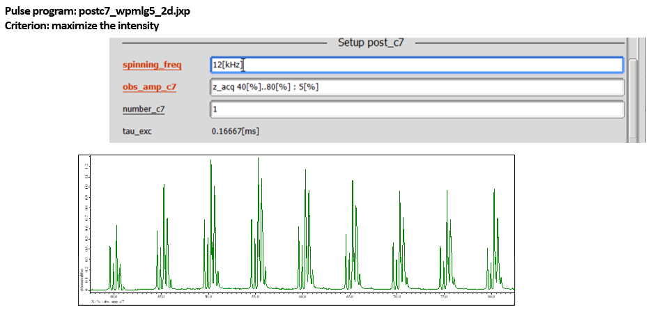
Fig 6.
DQ filtered 1H spectra of L-tyrosine.HCl at 12 kHz and 14.1 T observed at various rf field strength for POST-C7. The spectra were observed using the sequence in Fig 5 with t1 = 0. While nominal rf field strength for POST-C7 is seven times of the MAS rate, the maximum DQ efficiency may appear at the slightly different rf field strength.
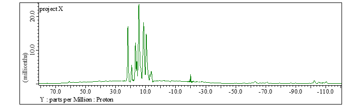
Fig 7.
Projection onto the DQ dimension of DQ/SQ correlation spectra of L-tyrosine.HCl at MAS rate of 12 kHz and 14.1T. POST-C7 is utilized to excite/reconvert DQ coherences. The DQ peaks appear not at the center but at +1 SSB positions.
Care must be taken for acquisition time. As rf field is almost continuously applied during excitation, t1, reconversion, and t2 period, the total duration has to be shorter than 50 ms to avoid probe failure. Be carefull of x_acq_time and y_acq_time.
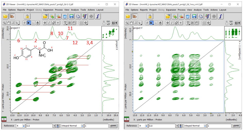
Fig 8.
1H DQ/1H SQ correlation spectra of L-tyrosine.HCl at 12 kHz MAS under 14.1 T without (a) and with (b, 1 ms) z-filtering. Internuclear connectivities are shown with red line in (a). Note that the 1H assignments are tentative.
1H DQ/ 1H SQ correlations: data processing (Fig 9)
The direct dimension is the same as 1D wPMLG. Linear_Ref and Reference should be applied to correct chemical shift scalings. In the indirect dimension, first peak position has to be shifted with a MAS rate as the peaks appear at +1 SSB (not at the center). This can be done by Reference function. Next Linier_Ref is applied to re-scale the chemical shift. Note that the spectral center is no longer at 50[%] since we applied reference at the first step. To correct this factor, Center should be set to x_offset * 2, which is automatically converted into numeric value depending on the experimental condition used. As the peak position is doubled in the DQ dimension, the parameter used in the subsequent Reference has to be doubled compared to the SQ dimension. Finally, diagonal line is drawn with a slope of 2.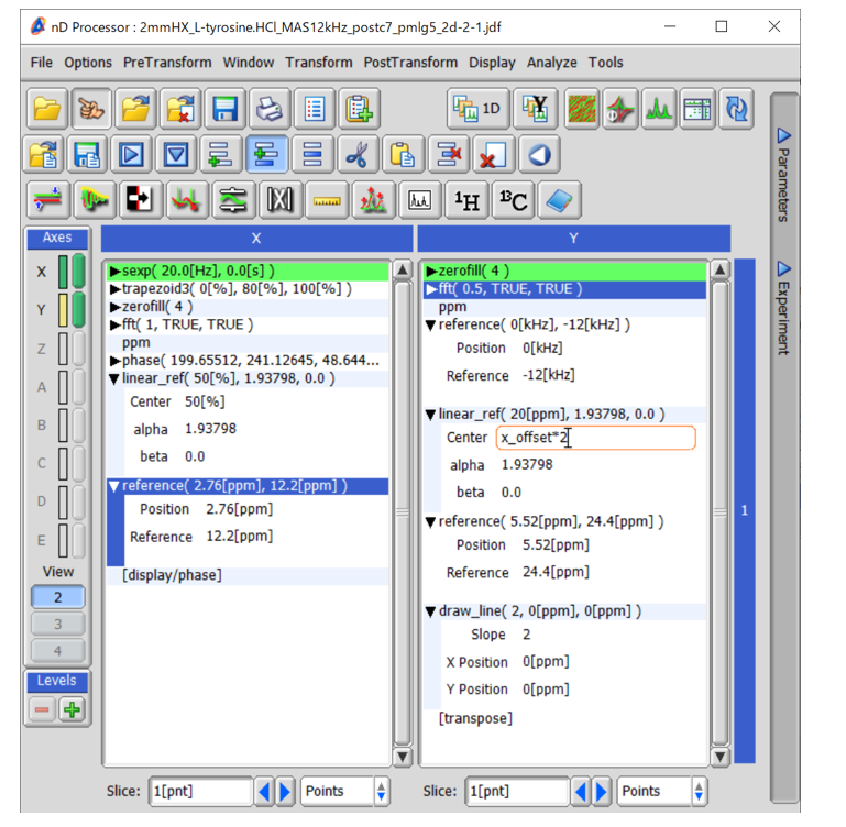
Fig 9.
Process list used in processing of 1H DQ/1H SQ correlation spectra of L-tyrosine.HCl at 12 kHz MAS under 14.1 T.
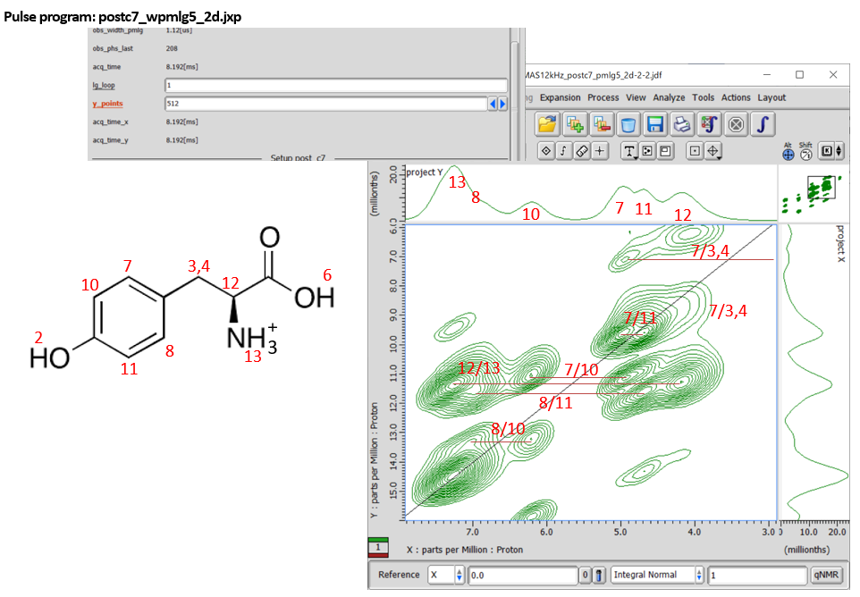
Fig 10.
Expansion of 1H DQ/1H SQ correlation spectra of L-tyrosine.HCl at 12 kHz MAS under 14.1 T. Whole spectrum is shown in Fig 8(a). Note that the 1H assignments are tentative. The increment of the indirect dimension is set to the wPMLG cycle time by putting Lg_loop = 1. 512 t1 points were collected with 12 cans for each. The total measurement time was 512 x 12 x 2 x 1.5 s (repetition delay) = 5.2 hours.
References:
- [1] S.P. Brown, Prog. Nucl. Magn. Reson. Spectrosc. 50 (2007) 199-251.
- [2] E. Salager, R.S. Stein, C.J. Pickard, B. Elena, L. Emsley, Phys. Chem. Chem. Phys. 11 (2009) 2610-2621.
- [3] J.-N. Dumez, M.C. Butler, E. Salager, B. Elena-Herrmann, L. Emsley, Phys. Chem. Chem. Phys. 12 (2010) 9172-9175.
- [4] N.T. Duong, S. Raran-Kurussi, Y. Nishiyama, V. Agarwal, J. Magn. Reson. 317 (2020) 106777.
- [5] H. Hohwy, H.J. Jakobsen, M. Eden, M.H. Levitt, N.C. Nielsen, J. Chem. Phys. 108 (1998) 2686-2694.
- [6] S.P. Brown, A. Lesage. B. Elena, L. Emsley, J. Am. Chem. Soc. 126 (2004) 13230-13231.
- [7] H. Geen, J.J. Titman, J. Gottwald, H.W. Spiess, J. Magn. Reson. A 114 (1995) 264-267.
- Please see the PDF file for the additional information.
Another window opens when you click. 
PDF 2,226KB
Related Products
Solutions by field
Are you a medical professional or personnel engaged in medical care?
No
Please be reminded that these pages are not intended to provide the general public with information about the products.